The Platypus framework provides us with a Python library to solve and analyze multi-objective problems conveniently. In this notebook, we use Platypus to solve a multi-objective optimization problem – the 3 objective version of DTLZ2 (Deb et al., 2002a) – using the evolutionary algorithm NSGA-II (Deb et al., 2002b). We generate runtime visualizations for snapshots of the algorithm to help build an understanding of how the evolutionary algorithm works. Specifically, we are going to look at the population at each generation, their ranks (a key parameter NSGA-II uses to select offspring), the parallel coordinates plot of the current population, and runtime indicators such as hypervolume and generational distance.
Setting up the problem
I created a Google Colab for this post. Since this post is equivalent to the Google Colab file, you may choose to look at either one. This project is intended to be used in a Jupyter Notebook environment with Python.
First, we import the Python libraries we need for the visualization.
import numpy as np
import math
import pandas as pd
from pandas.plotting import parallel_coordinates
import random
from tqdm.notebook import tqdm

import matplotlib.pyplot as plt
from matplotlib import animation, rc, rcParams
rc('animation', html='jshtml')

from mpl_toolkits.mplot3d import Axes3D

!pip install platypus-opt
from platypus import (NSGAII, NSGAIII, DTLZ2, Hypervolume, EpsilonBoxArchive,
                      Solution, GenerationalDistance, InvertedGenerationalDistance,
                      Hypervolume, EpsilonIndicator, Spacing)
Our goal is to visualize the population at each generation of the evolutionary algorithm. To do so, we utilize an interface provided by the Platypus library: the callback function.
At each iteration of the algorithm, the callback function (if initialized) is called. We define our callback function to store the current number of function evaluations (algorithm.nfe) and all the data points in the current population (algorithm.result). Each population has the type Solution defined in Platypus, which not only contains the values of the variables but also attributes specific to the solver, such as ranks and crowding distances. We will access some of these attributes during visualization.
We also define the frequency of NFEs that we want to store the values. Saving a snapshot of the algorithm at every single iteration may be too expensive or unnecessary. Hence, we set a lapse for some number of iterations, in which the callback function does nothing unless the last NFE is more than the frequency amount apart from this NFE.
In the following example, we set up the problem DTLZ2 and use the callback function to solve it using NSGAII.
#define the frequency
frequency = 200

# define the problem definition
problem = DTLZ2(3)

# instantiate the optimization algorithm
algorithm = NSGAII(problem, divisions_outer=12)

# define callback function
solutions_list = []
hyp = []
nfe = []
last_calc = 0

def DTLZ2_callback(algorithm):
  global last_calc
  if algorithm.nfe == last_calc + frequency:
    last_calc = algorithm.nfe
    nfe.append(algorithm.nfe)
    solutions_list.append(algorithm.result);

# optimize the problem using 10,000 function evaluations
algorithm.run(10000,DTLZ2_callback)
In order to calculate the metrics, we first need to define our reference set. For DTLZ2(3), our points lie on the unit sphere in the first octant. Let’s randomly select 1000 such points and plot them.
# generate the reference set for 3D DTLZ2
reference_set = EpsilonBoxArchive([0.02, 0.02, 0.02])

for _ in range(1000):
    solution = Solution(problem)
    solution.variables = [random.uniform(0,1) if i < problem.nobjs-1 else 0.5 for i in range(problem.nvars)]
    solution.evaluate()
    reference_set.add(solution)

fig_ref = plt.figure()
ax_ref = fig_ref.add_subplot(projection="3d")
ax_ref.scatter(
              [s.objectives[0] for s in reference_set],
              [s.objectives[1] for s in reference_set],
              [s.objectives[2] for s in reference_set],
              )
Given the reference set, we can now calculate the indicators for each population across iterations. The Platypus library provides us with all the functions we need to calculate the following indicators: generational distance, hypervolume, epsilon indicator, and spacing.
We initialize them in a dictionary and iterate over all saved populations to calculate the indicators.
# calculate the indicators
indicators = {"gd" : GenerationalDistance(reference_set),
              "hyp" : Hypervolume(reference_set),
              "ei" : EpsilonIndicator(reference_set),
              "sp" : Spacing()}

indicator_results = {index : [] for index in indicators}

for indicator in tqdm(indicator_results):
  for solution in tqdm(solutions_list):
    indicator_results[indicator] += [indicators[indicator].calculate(solution)]
Setting up the visualization
At this point, we have the data we need to perform runtime visualizations. We will utilize the animation.FuncAnimation function in matplotlib to create interactive animations in Jupyter Notebook (or Google Colab). The idea behind creating such animations is to first initialize a static figure, and then define an update function to let the FuncAnimation know how to visualize new data for each iteration.
We define drawframe() that does the following: (1) clear the axis, so that previous data points are wiped out; (2) draw the new data points; (3) reset the limits of data axes so that the axes are consistent across frames; (4) update new data for indicator axes.
def drawframe(n):

    # clear axes
    ax.cla()
    ax_parallel.cla()

    # save results
    result = solutions_list[n]
    crowding_distances = [s.crowding_distance if s.crowding_distance != math.inf else 0 for s in result]
    ranks = [s.rank for s in result]

    result = solutions_list[n]
    points = {
              'X': [s.objectives[0] for s in result],
              'Y': [s.objectives[1] for s in result],
              'Z': [s.objectives[2] for s in result],
              'rank': [s.rank for s in result],
              'tag' : ['tag' for s in result]
    }
    df = pd.DataFrame(points)

    # update new data points
    ax.scatter(points['X'], points['Y'], points['Z'],
              c = ranks,
              alpha = 0.5,
              linestyle="", marker="o",
              cmap=cmap,
              vmax=max_rank,
              vmin=0)
    ax.set_xlim(xlim)
    ax.set_ylim(ylim)
    ax.set_zlim(zlim)
    ax.set_title('Solve DTLZ2, NFE = ' + str(nfe[n]))

    # update the parallel coordinates plot
    parallel_coordinates(df[['X','Y','Z','tag']], 'tag', ax=ax_parallel)

    # update indicator plots
    for indicator in indicator_axes:
      indicator_ax = indicator_axes[indicator]
      indicator_ax.plot(nfe[:n],indicator_results[indicator][:n], c = 'r')
      indicator_ax.set_xlim(left = min(nfe), right=max(nfe))
      indicator_ax.set_ylim(bottom = min(indicator_results[indicator]), top = max(indicator_results[indicator]))
With the drawframe() function, we create a static figure that initializes the axes we will feed into the drawframe() function. The initialization does the following: (1) set up the subplots of the figure; (2) calculate the maximum ranks of all points in all populations to determine the color mapping; (3) load the points from the first iteration; (4) initialize the scatter plots, parallel coordinates plot, and indicator plots.
fig = plt.figure(figsize=(20,10), dpi = 70)
fig.suptitle("Runtime Visualization", fontsize=20)
fig.subplots_adjust(wspace=0.3, hspace=0.3)
ax = fig.add_subplot(2, 3, 1, projection="3d")
ax_parallel = fig.add_subplot(2,3,4)

indicator_axes = {"gd" : fig.add_subplot(2, 3, 2),
                  "hyp" : fig.add_subplot(2, 3, 3),
                  "ei" : fig.add_subplot(2, 3, 5),
                  "sp" : fig.add_subplot(2, 3, 6)}

indicator_names = {"gd" : "Generational Distance",
                  "hyp" : "Hypervolume",
                  "ei" : "Epsilon Indicator",
                  "sp" : "Spacing"}

# load the ranks of all points
all_rank = [s.rank for result in solutions_list for s in result]
max_rank = max(all_rank)

# define the colormap
cmap = plt.get_cmap('Accent', max_rank)

# load the points from the first iteration
result = solutions_list[0]
points = {
    'X': [s.objectives[0] for s in result],
    'Y': [s.objectives[1] for s in result],
    'Z': [s.objectives[2] for s in result],
    'rank': [s.rank for s in result],
    'tag' : ['tag' for s in result]
}

df = pd.DataFrame(points)

# create the scatter plot
graph = ax.scatter(
              points['X'], points['Y'], points['Z'],
              c = points['rank'],
              alpha = 0.5,
              cmap=cmap,
              linestyle="", marker="o",
              vmax=max_rank,
              vmin=0
          )

# create the parallel coordinates plot
parallel_coordinates(df[['X','Y','Z','tag']], 'tag', ax=ax_parallel)

plt.colorbar(graph, label='Rank', pad = 0.2)

# save the dimensions for later use
xlim = ax.get_xlim()
ylim = ax.get_ylim()
zlim = ax.get_zlim()
title = ax.set_title("DTLZ2 Static Figure")
ax.set_xlabel("x")
ax.set_ylabel("y")
ax.set_zlabel("z")

# initialize subplots for each indicator
for indicator in indicator_axes:
  indicator_axes[indicator].plot(nfe[:0],indicator_results[indicator][:0])
  indicator_axes[indicator].set_title(indicator_names[indicator] + " vs NFE")
  indicator_axes[indicator].set_xlabel("NFE")
  indicator_axes[indicator].set_ylabel(indicator_names[indicator])
Now we are ready to create an animation. We use the FuncAnimation() function, the initialized figure, and the drawframe() function to create the animation.
In the Jupyter Notebook or Google Colab, you will be able to play the animation using the play button at the bottom of the image. By default, the animation will play in a loop. You may select “once” so that the animation freezes in the last frame. Important: Before re-generating the animation, be sure to re-run the previous initialization so that the figure is reset. Otherwise, you may see overlapping points/lines.
ani = animation.FuncAnimation(fig, drawframe, frames=len(nfe), interval=20, blit=False)
ani
This visualization shows how the algorithm progresses as NFE grows. For the set of solutions, we clearly see how they converge to the reference set. Moreover, more and more points have lower ranks, indicating they are getting closer to the Pareto Front (points on the Pareto Front have rank = 0). The parallel coordinates plot shows how our solutions get narrowed down and the tradeoffs we could make. Finally, the four indicator plots track the performance of our algorithm as NFE increases. The trajectory of generational distance, hypervolume, and epsilon indicator suggests convergence.
In conclusion, the project highlights the potential of the Platypus library in Python in providing valuable insights into the progress of evolutionary algorithms, not just their final outcomes. Through the use of NSGA-II as an illustrative example, we have demonstrated the ability to monitor the ranks of points across generations. In Dave’s post, the runtime visualizations revealed the changing probabilities of variators across iterations. These findings emphasize the power of incorporating dynamic techniques to gain a comprehensive understanding of the runtime behavior of MOEA algorithms. I hope this project opens doors to further explore, visualize, and analyze the dynamics of evolutionary algorithms.
References
[1] Deb, K., Thiele, L., Laumanns, M., & Zitzler, E. (2002a). Scalable multi-objective optimization test problems. In Proceedings of the 2002 Congress on Evolutionary Computation. CEC’02 (Cat. No. 02TH8600) (Vol. 1, pp. 825-830). IEEE.
[2] Deb, K., Pratap, A., Agarwal, S., & Meyarivan, T. A. M. T. (2002b). A fast and elitist multiobjective genetic algorithm: NSGA-II. IEEE transactions on evolutionary computation, 6(2), 182-197.
I’ve been developing some course material on multiobjective optimization, and I thought I’d share an introductory exercise I’ve written as a blog post. The purpose of the exercise is to introduce students to multi-objective optimization, starting with basic terms and moving toward the central concept of Pareto dominance (which I’ll define below). The exercise explores trade-offs across two conflicting objectives in the design of a cantilever beam. This example is drawn from the textbook “Multi-Objective Optimization using Evolutionary Algorithms” by Kalyanmoy Deb (2001), though all code is original. This exercise is intended to be a teaching tool to complement introductory lectures on multi-objective optimization and Pareto dominance.
A simple model of a cantilever beam
In this exercise, we’ll first develop a simple model to evaluate a cantilever beam’s deflection, weight, and stress supporting a constant force (as specified by Deb, 2001). We’ll then enumerate possible design alternatives and visualize feasible designs and their performance. Next, we’ll introduce Pareto Dominance and examine trade-offs between conflicting system objectives. Finally, we’ll use the NSGA-II Multiobjective Evolutionary Algorithm (MOEA) to discover a Pareto-approximate set of designs and visualize design alternatives.
Let’s start by considering the cantilever beam shown below.
Our task is to “design” the beam by specifying its length (l) and diameter (d). Assuming the beam will be subjected to a constant force, P, we are interested in minimizing two conflicting performance objectives, the weight and the end deflection. We can model our beam using the following system of equations:
Following Deb (2001), we’ll use the parameter values shown below:
10mm ≤ d ≤ 50 mm; 200 mm ≤ l ≤ 1000 mm; ρ = 7800 kg/m3; P = 1 KN; E = 207 GPa
We would also like to ensure that our beam meets two feasibility constraints:
Modeling the beam in Python
As multiobjective design problems go, this is a fairly simple problem to solve. We can enumerate all possible design options and explore trade-offs between different combinations of length and diameter. Below I’ve coded a Python function to evaluate a beam with parameters l and d.
# create a model of the beam
def cantileverBeam(l, d):
    """
    Models the weight, deflection and stress on a cantilever beam subjected to a force of P=1 kN
    :param l:           length of the beam (mm)
    :param d:           diameter of the beam (mm)
    :return:
        - weight: the weight of the beam
        - deflection: the deflection of the beam
        - stress: the stress on the beam
    """

    weight = (7800.0 * (3.14159 * d**2)/4 * l)/1000000000 # (division by 1000000000 is unit conversion)
    deflection = (64.0*P * l**3)/(3.0*207.0*3.14159*d**4)
    stress = (32.0 * P * l)/(3.14159*d**3)

    return weight, deflection, stress
With this function, we can explore alternative beam designs. We’ll first create a set of samples of l and d, then simulate them through our beam model. Using our results, we’ll visualize the search space, which includes all possible design alternatives for l and d, enclosed 10≤ d ≤ 50 and 200 ≤ l ≤ 1000. Inside the search space, we can also delineate the feasible decision space composed of all combinations of l and d that meet our beam performance constraints. Every feasible solution can be mapped to the feasible objective space, which contains each sized beam’s corresponding weight and deflection. In the code below, we’ll simulate 1681 different possible beam designs and visualize the feasible decision space and the corresponding objective space.
import numpy as np
from matplotlib import pyplot as plt

# initialize arrays to store our design parameters
l = np.arange(200, 1020, 20)
d = np.arange(10,51,1)
P = 1.0

# initialize arrays to store model output
weight = np.zeros([41,41])
deflection = np.zeros([41,41])
constraints = np.zeros([41,41])
stress = np.zeros([41,41])

# evaluate the system
for i in range(41):
    for j in range(41):
        weight[i, j], deflection[i,j], stress[i,j] = cantileverBeam(l[i], d[j])
        if stress[i, j] <= 300 and deflection[i, j] <= 5:
            constraints[i,j] =1

# create a figure with two subplots
fig, axes = plt.subplots(1, 2, figsize=(12,4))

# plot the decision space
for i in range(41):
    for j in range(41):
        axes[0].scatter(i,j, c=constraints[i,j], cmap='Blues', vmin=0, vmax=1, alpha=.6)
axes[0].set_xticks(np.arange(0,45,5))
axes[0].set_yticks(np.arange(0,45,5))
axes[0].set_yticklabels(np.arange(10,55,5))
axes[0].set_xticklabels(np.arange(200,1100,100))
axes[0].set_xlabel('Length (mm)')
axes[0].set_ylabel('Diameter (mm)')
axes[0].set_title('Decision Space')

# plot the objective space
axes[1].scatter(weight.flatten(), deflection.flatten(), edgecolor='white')
axes[1].set_ylim([0,5])
axes[1].set_xlabel('Weight (kg)')
axes[1].set_ylabel('Deflection (mm)')
axes[1].set_title('Objective Space')
Examining the figures above, we observe that only around 40% of our evaluated beam designs are feasible (they meet the constraints of maximum stress and deflection). We can see a clear relationship between length and diameter – long narrow beams are unlikely to meet our constraints. When we examine the objective space of feasible beam designs, we observe trade-offs between our two objectives, weight and deflection. Examine the objective space. Is there a clear “best” beam that you would select? Are there any alternatives that you would definitely not select?
Introducing Pareto Dominance
Without a clear articulation of our preferences between weight and deflection, we cannot choose a single “best” design. We can, however, definitively rule out many of the beam designs using the concept of Pareto dominance. We’ll start by picking and comparing the objectives of any two designs from our set of feasible alternatives. For some pairs, we observe that one design is better than the other in both weight and deflection. In this case, the design that is preferable in both objectives is said to dominate the other design. For other pairs of designs, we observe that one design is preferable in weight while the other is preferable in deflection. In this case, both designs are non-dominated, meaning that the alternative is not superior in both objectives. If we expand from pairwise comparisons to evaluating the entire set of feasible designs simultaneously, we can discover a non-dominated set of designs. We call this set of designs the Pareto-optimal set. In our beam design problem, this is the set of designs that we should focus our attention on, as all other designs are dominated by at least one member of this set. The curve made by plotting the Pareto-optimal set is called the Pareto front. The Pareto front for the problem is plotted in orange in the figure below.
Multiobjective optimization
As mentioned above, the cantilever beam problem is trivial because we can easily enumerate all possible solutions and manually find the Pareto set. However, we are not so lucky in most environmental and water resources applications. To solve more challenging problems, we need new tools. Fortunately for us, these tools exist and have been rapidly improving in recent decades (Reed et al., 2013). One family of multiobjective optimization techniques that have been shown to perform well on complex problems is MOEAs (Coello Coello, 2007). MOEAs use search operators inspired by natural evolution, such as recombination and mutation, to “evolve” a population of solutions and generate approximations of the Pareto set. In the sections below, we’ll employ a widely used MOEA, NSGA-II (Deb et al., 2002), to find Pareto approximate designs for our simple beam problem. We’ll use the Platypus Python library to implement our evolutionary algorithm and explore results. Platypus is a flexible and easy-to-use library that contains 20 different evolutionary algorithms. For more background on MOEAs and Platypus, see the examples in the library’s online documentation.
Formulating the optimization problem
Formally, we can specify our multiobjective problem as follows:
Multiobjective optimization in Python with Platypus
Below we’ll define a function to use in Platypus based on our problem formulation. To work with Platypus, this function must accept a vector of decision variables (called vars) and return a vector of objectives and constraints.
# Define a function to use with NSGA-II
def evaluate_beam(vars):
    """
    A version of the cantilever beam model to optimize with an MOEA in Platypus

    :param vars:        a vector with decision variables element [0] is length, [1] is diameter
    :return:
        - a vector of objectives [weight, deflection]
        - a vector of constraints, [stress, deflection]

    """
    l = vars[0]
    d = vars[1]

    weight = (7800.0 * (3.14159 * d ** 2) / 4 * l)/1000000000
    deflection = (64.0*1.0 * l**3)/(3.0*207.0*3.14159*d**4)
    stress = (32.0 * 1.0 * l)/(3.14159*d**3)

    return [weight, deflection], [stress - 300, deflection - 5]
Next, we’ll instantiate a problem class in Platypus. We’ll first create a class with 2 decision variables, 2 objectives, and 2 constraints, then specify the allowable range of each decision variable, the type of constraints, and s function the algorithm will evaluate. We’ll then select NSGAII as our algorithm and run the optimization for 1000 generations.
# set up the Platypus problem (2 decision variables, 2 objectives, 2 constraints)
problem = Problem(2, 2, 2)

# specify the decision variable ranges (200 mm <= length <= 1000 mm) and (10 mm <= diameter <= 50 mm)
problem.types[:] = [Real(200, 1000), Real(10, 50)]

# specify the type of constraint
problem.constraints[:] = "<=0"

# tell Platypus what function to optimize
problem.function = evaluate_beam

# set NSGA II to optimize the problem
algorithm = NSGAII(problem)

# run the optimization for 1000 generations
algorithm.run(2000)
Plotting our approximation of the Pareto front allows us to examine trade-offs between the two conflicting objectives.
# plot the Pareto approximate set
fig = plt.figure()
plt.scatter([s.objectives[0] for s in algorithm.result],
            [s.objectives[1] for s in algorithm.result])
plt.xlabel('Weight (kg)')
plt.ylabel('Deflection (mm)')
plt.xlim([0,5])
plt.ylim([0,5])
NSGA-II has found a set of non-dominated designs that show a strong trade-off between beam weight and deflection. But how does our approximation compare to the Pareto front we discovered above? A good approximation of the Pareto front should have two properties 1) convergence, meaning the approximation is close to the true Pareto front, and 2) diversity, meaning the solutions cover as much of the true Pareto front as possible. We can plot the designs discovered by NSGA-II in the space of the enumerated designs to reveal that the algorithm is able to do a great job approximating the true Pareto front. The designs it discovered are right on top of the true Pareto front and maintain good coverage of the range of trade-offs.
In real-world design problems, the true Pareto front is usually not known, so it’s important to evaluate an MOEA run using runtime diagnostics to assess convergence. Here we can visualize the algorithm’s progress over successive generations to see it converge to a good approximation of the Pareto front. Notice how the algorithm first evolves solutions that maintain good convergence, then adds to these solutions to find a diverse representation of the Pareto front. In more complex or higher-dimensional contexts, metrics of runtime performance are required to assess MOEA performance. For background on runtime diagnostics and associated performance metrics, see this post.
Final thoughts
In this exercise, we’ve explored the basic multiobjective concepts through the design of a cantilever beam. We introduced the concepts of the search space, feasible decision space, objective space, and Pareto dominance. We also solved the multiobjective optimization problem using the NSGA-II MOEA. While the cantilever beam model used here is simple, our basic design approach can be adapted to much more complex and challenging problems.
References
Coello, C. C. (2006). Evolutionary multi-objective optimization: a historical view of the field. IEEE computational intelligence magazine, 1(1), 28-36.
Deb, K. (2011). Multi-objective optimisation using evolutionary algorithms: an introduction. In Multi-objective evolutionary optimisation for product design and manufacturing (pp. 3-34). London: Springer London.
Deb, K., Pratap, A., Agarwal, S., & Meyarivan, T. A. M. T. (2002). A fast and elitist multiobjective genetic algorithm: NSGA-II. IEEE transactions on evolutionary computation, 6(2), 182-197.
Reed, P. M., Hadka, D., Herman, J. D., Kasprzyk, J. R., & Kollat, J. B. (2013). Evolutionary multiobjective optimization in water resources: The past, present, and future. Advances in water resources, 51, 438-456.
Welcome to the second post in the Fisheries Training Series, in which we are studying decision making under deep uncertainty within the context of a complex harvested predator-prey fishery. The accompanying GitHub repository, containing all of the source code used throughout this series, is available here. The full, in-depth Jupyter Notebook version of this post is available in the repository as well.
A brief re-cap of the harvested predator-prey model
Formulation of the harvesting policy and an overview of radial basis functions (RBFs)
Formulation of the policy objectives
A simulation model for the harvested system
Optimization of the harvesting policy using the PyBorg MOEA
Installation of Platypus and PyBorg*
Optimization problem formulation
Basic MOEA diagnostics
Note *The PyBorg MOEA used in this demonstration is derived from the Borg MOEA and may only be used with permission from its creators. Fortunately, it is freely available for academic and non-commercial use. Visit BorgMOEA.org to request access.
Now, onto the tutorial!
Harvested predator-prey model
In the previous post, we introduced a modified form of the Lotka-Volterra system of ordinary differential equations (ODEs) defining predator-prey population dynamics.
This modified version includes a non-linear predator population growth dynamic original proposed by Arditi and Akçakaya (1990), and includes a harvesting parameter, . This system of equations is defined in Hadjimichael et al. (2020) as:
Where is the prey population being harvested and is the predator population. Please refer to Post 0 of this series for the rest of the parameter descriptions, and for insights into the non-linear dynamics that result from these ODEs. It also demonstrates how the system alternates between ‘basins’ of stability and population collapse.
Harvesting policy
In this post, we instead focus on the generation of harvesting policies which can be operated safely in the system without causing population collapse. Rather than assigning a deterministic (specific, pre-defined) harvest effort level for every time period, we instead design an adaptive policy which is a function of the current state of the system:
The problem then becomes the optimization of the control rule, , rather than specific parameter values, . The process of optimizing the parameters of a state-aware control rule is known as Direct Policy Search (DPS; Quinn et al, 2017).
Previous work done by Quinn et al. (2017) showed that an adaptive policy, generated using DPS, was able to navigate deeply uncertain ecological tipping points more reliably than intertemporal policies which prescribed specific efforts at each timestep.
Radial basis functions
The core of the DPS method are radial basis functions (RBFs), which are flexible, parametric function formulations that map the current state of the system to policy action. A previous study by Giuliani et al (2015) demonstrated that RBFs are highly effective in generating Pareto-approximate sets of solutions, and that they perform well when applied to horizons different from the optimized simulation horizon.
There are various RBF approaches available, such as the cubic RBF used by Quinn et al. (2017). Here, we use the Gaussian RBF introduced by Hadjimichael et al. (2020), where the harvest effort during the next timestep, , is mapped to the current prey population levels, by the function:
In this formulation and are the center, radius, and weights of each RBF respectively. Additionally, is the number of RBFs used in the function; in this study we use RBFs. With two RBFs, there are a total of 6 parameters. Increasing the number of RBFs allows for more flexible function forms to be achieved. However, two RBFs have been shown to be sufficient for this problem.
The sum of the weights must be equal to one, such that:
The function harvest_streategy() is contained within the fish_game_functions.py script, which can be accessed here in the repository.
A simplified rendition of the harvest_strategy() function, evaluate_RBF(), is shown below and uses the RBF parameter values (i.e., ), and the current prey population, to calculate the next year’s harvesting effort.
import numpy as np
import matplotlib.pyplot as plt

def evaluate_RBF(x, RBF_params, nRBFs):
    """
    Parameters:
    -----------
    x : float
        The current state of the system.
    RBF_params : list [3xnRBFs]
        The RBF parameters in the order of [c, r, w,...,c, r, w].
    nRBFs : int
        The number of RBFs used in the mapping function.

    Returns:
    --------
    z : float
        The policy action.
    """

    c = RBF_params[0::3]
    r = RBF_params[1::3]
    w = RBF_params[2::3]

    # Normalize the weights
    w_norm = []
    if np.sum(w) != 0:
        for w_i in w:
            w_norm.append(w_i / np.sum(w))
    else:
        w_norm = (1/nRBFs)*np.ones(len(w))

    z = 0.0

    for i in range(nRBFs):

        # Avoid division by zero
        if r[i] != 0:
            z = z + w[i] * np.exp(-((x - c[i])/r[i])**2)
        else:
            z = z + w[i] * np.exp(-((x - c[i])/(10**-6))**2)

    # Impose limits on harvest effort
    if z < 0:
        z = 0
    elif z > 1:
        z = 1

    return z
To better understand the nature of the harvesting policy, it is helpful to visualize the policy function, .
For some arbitrary selection of RBF parameters:
The following function will plot the harvesting strategy:
def plot_RBF_policy(x_range, x_label, y_range, y_label, RBF_params, nRBFs):
    """
    Parameters:
    -----------
    RBF_params : list [3xnRBFs]
        The RBF parameters in the order of [c, r, w,...,c, r, w].
    nRBFs : int
        The number of RBFs used in the mapping function.

    Returns:
    --------
    None.
    """
    # Step size
    n = 100
    x_min = x_range[0]
    x_max = x_range[1]
    y_min = y_range[0]
    y_max = y_range[1]

    # Generate data
    x_vals = np.linspace(x_min, x_max, n)
    y_vals = np.zeros(n)

    for i in range(n):
        y = evaluate_RBF(x_vals[i], RBF_params, nRBFs)

        # Check that assigned actions are within range
        if y < y_min:
            y = y_min
        elif y > y_max:
            y = y_max

        y_vals[i] = y

    # Plot
    fig, ax = plt.subplots(figsize = (5,5), dpi = 100)
    ax.plot(x_vals, y_vals, label = 'Policy', color = 'green')
    ax.set_xlabel(x_label)
    ax.set_ylabel(y_label)
    ax.set_title('RBF Policy')
    plt.show()
    return
Let’s take a look at the policy that results from the random RBF parameters listed above. Setting my problem-specific inputs, and running the function:
This policy does not make much intuitive sense… why should harvesting efforts be decreased when the fish population is large? Well, that’s because we chose these RBF parameter values randomly.
To demonstrate the flexibility of the RBF functions and the variety of policy functions that can result from them, I generated a few (n = 7) policies using a random sample of parameter values. The parameter values were sampled from a uniform distribution over each parameters range: . Below is a plot of the resulting random policy functions:
Fig: Many random RBF policies, showing flexibility of RBFs.
Finding the sets of RBF parameter values that result in Pareto-optimal harvesting policies is the next step in this process!
Harvest strategy objectives
We take a multi-objective approach to the generation of a harvesting strategy. Given that the populations are vulnerable to collapse, it is important to consider ecological objectives in the problem formulation.
Here, we consider five objectives, described below.
Objective 1: Net present value
The net present value (NPV) is an economic objective corresponding to the amount of fish harvested.
During the simulation-optimization process (later in this post), we simulate a single policy times, and take the average objective score over the range of simulations. This method helps to account for variability in expected outcomes due to natural stochasticity. Here, we use realizations of stochasticity.
With that in mind, the NPV () is calculated as:
where is the discount rate which converts future benefits to present economic value, here .
Objective 2: Prey population deficit
The second objective aims to minimize the average prey population deficit, relative to the prey population carrying capacity, :
Objective 3: Longest duration of consecutive low harvest
In order to maintain steady harvesting levels, we minimize the longest duration of consecutive low harvests. Here, a subjective definition of low harvest is imposed. In a practical decision making process, this threshold may be solicited from the relevant stakeholders.
Objective 3 is defined as:
where
And the low harvest limit is: .
Objective 4: Worst harvest instance
In addition to avoiding long periods of continuously low harvest, the stakeholders have a desire to limit financial risks associated with very low harvests. Here, we minimize the worst 1% of harvest.
The fourth objective is defined as:
Objective 5: Harvest variance
Lastly, policies which result in low harvest variance are more easily implemented, and can limit corresponding variance in fish populations.
The last objective minimizes the harvest variance, with the objective score defined as:
Constraint: Avoid collapse of predator population
During the optimization process, we are able to include constraints on the harvesting policies.
Since population collapse is a stable equilibrium point, from which the population will not regrow, it is imperative to consider policies which prevent collapse.
With this in mind, the policy must not result in any population collapse across the realizations of environmental stochasticity. Mathematically, this is enforced by:
where
Problem formulation
Given the objectives described above, the optimization problem is:
Simulation model of the harvested system
Here, we provide an overview of the fish_game_5_objs() model which combines many of the preceding topics. The goal for this model is to take a set of RBF parameters, which define the harvesting strategy, simulate the policy for some length of time, and then return the objective scores resulting from the policy.
Later, this model will allow for the optimization of the harvesting policy RBF parameters through a Multi-Objective Evolutionary Algorithm (MOEA). The MOEA will evaluate many thousands of policies (RBF parameter combinations) and attempt to find, through evolution, those RBF parameters which yield best objective performance.
A brief summary of the model process is described here, but the curious learner is encouraged to take a deeper look at the code and dissect the process.
The model can be understood as having three major sections:
Initialization of storage vectors, stochastic variables, and assumed ODE parameters.
Simulation of policy and fishery populations over time period T.
Calculation of objective scores.
def fish_game_5_objs(vars):
    """
    Defines the full, 5-objective fish game problem to be solved

    Parameters
    ----------
    vars : list of floats
        Contains the C, R, W values

    Returns
    -------
    objs, cnstr
    """

    # Get chosen strategy
    strategy = 'Previous_Prey'

    # Define variables for RBFs
    nIn = 1 # no. of inputs (depending on selected strategy)
    nOut = 1 # no. of outputs (depending on selected strategy)
    nRBF = 2 # no. of RBFs to use

    nObjs = 5
    nCnstr = 1 # no. of constraints in output

    tSteps = 100 # no. of timesteps to run the fish game on
    N = 100 # Number of realizations of environmental stochasticity

    # Define assumed system parameters
    a = 0.005
    b = 0.5
    c = 0.5
    d = 0.1
    h = 0.1
    K = 2000
    m = 0.7
    sigmaX = 0.004
    sigmaY = 0.004

    # Initialize storage arrays for populations and harvest
    x = np.zeros(tSteps+1) # Prey population
    y = np.zeros(tSteps+1) # Predator population
    z = np.zeros(tSteps+1) # Harvest effort

    # Create array to store harvest for all realizations
    harvest = np.zeros([N,tSteps+1])
    # Create array to store effort for all realizations
    effort = np.zeros([N,tSteps+1])
    # Create array to store prey for all realizations
    prey = np.zeros([N,tSteps+1])
    # Create array to store predator for all realizations
    predator = np.zeros([N,tSteps+1])

    # Create array to store metrics per realization
    NPV = np.zeros(N)
    cons_low_harv = np.zeros(N)
    harv_1st_pc = np.zeros(N)
    variance = np.zeros(N)

    # Create arrays to store objectives and constraints
    objs = [0.0]*nObjs
    cnstr = [0.0]*nCnstr

    # Create array with environmental stochasticity for prey
    epsilon_prey = np.random.normal(0.0, sigmaX, N)

    # Create array with environmental stochasticity for predator
    epsilon_predator = np.random.normal(0.0, sigmaY, N)

    # Go through N possible realizations
    for i in range(N):

        # Initialize populations and values
        x[0] = prey[i,0] = K
        y[0] = predator[i,0] = 250
        z[0] = effort[i,0] = harvest_strategy([x[0]], vars, [[0, K]], [[0, 1]], nIn, nOut, nRBF)
        NPVharvest = harvest[i,0] = effort[i,0]*x[0]

        # Go through all timesteps for prey, predator, and harvest
        for t in range(tSteps):

            # Solve discretized form of ODE at subsequent time step
            if x[t] > 0 and y[t] > 0:
                x[t+1] = (x[t] + b*x[t]*(1-x[t]/K) - (a*x[t]*y[t])/(np.power(y[t],m)+a*h*x[t]) - z[t]*x[t])* np.exp(epsilon_prey[i]) # Prey growth equation
                y[t+1] = (y[t] + c*a*x[t]*y[t]/(np.power(y[t],m)+a*h*x[t]) - d*y[t]) *np.exp(epsilon_predator[i]) # Predator growth equation

                # Solve for harvesting effort at next timestep
                if t <= tSteps-1:
                    if strategy == 'Previous_Prey':
                        input_ranges = [[0, K]] # Prey pop. range to use for normalization
                        output_ranges = [[0, 1]] # Range to de-normalize harvest to
                        z[t+1] = harvest_strategy([x[t]], vars, input_ranges, output_ranges, nIn, nOut, nRBF)

            # Store values in arrays
            prey[i,t+1] = x[t+1]
            predator[i,t+1] = y[t+1]
            effort[i,t+1] = z[t+1]
            harvest[i,t+1] = z[t+1]*x[t+1]
            NPVharvest = NPVharvest + harvest[i,t+1]*(1+0.05)**(-(t+1))

        # Solve for objectives and constraint
        NPV[i] = NPVharvest
        low_hrv = [harvest[i,j]<prey[i,j]/20 for j in range(len(harvest[i,:]))] # Returns a list of True values when there's harvest below 5%
        count = [ sum( 1 for _ in group ) for key, group in itertools.groupby( low_hrv ) if key ] # Counts groups of True values in a row
        if count: # Checks if theres at least one count (if not, np.max won't work on empty list)
            cons_low_harv[i] = np.max(count)  # Finds the largest number of consecutive low harvests
        else:
            cons_low_harv[i] = 0
        harv_1st_pc[i] = np.percentile(harvest[i,:],1)
        variance[i] = np.var(harvest[i,:])

    # Average objectives across N realizations
    objs[0] = -np.mean(NPV) # Mean NPV for all realizations
    objs[1] = np.mean((K-prey)/K) # Mean prey deficit
    objs[2] = np.mean(cons_low_harv) # Mean worst case of consecutive low harvest across realizations
    objs[3] = -np.mean(harv_1st_pc) # Mean 1st percentile of all harvests
    objs[4] = np.mean(variance) # Mean variance of harvest

    cnstr[0] = np.mean((predator < 1).sum(axis=1)) # Mean number of predator extinction days per realization

    # output should be all the objectives, and constraint
    return objs, cnstr
The next section shows how to optimize the harvest policy defined by vars, using the PyBorg MOEA.
A (Very) Brief Overview of PyBorg
PyBorg is the secondary implementation of the Borg MOEA written entirely in Python by David Hadka and Andrew Dircks. It is made possible using functions from the Platypus optimization library, which is a Python evolutionary computing framework.
As PyBorg is Borg’s Python wrapper and thus derived from the original Borg MOEA, it can only be used with permission from its creators. To obtain permission for download, please visit BorgMOEA and complete the web form. You should receive an email with the link to the BitBucket repository shortly.
Installation
The repository you have access to should be named ‘Serial Borg MOEA’ and contain a number of folders, including one called Python/. Within the Python/ folder, you will be able to locate a folder called pyborg. Once you have identified the folder, please follow these next steps carefully:
Check your current Python version. Python 3.5 or later is required to enable PyBorg implementation.
Download the pyborg folder and place it in the folder where this Jupyter Notebook all other Part 1 training material is located.
Install the platypus library. This can be in done via your command line by running one of two options:
Make sure the following training startup files are located within the same folder as this Jupyter Notebook: a) fish_game_functions.py: Contains all function definitions to setup the problem, run the optimization, plot the hypervolume, and conduct random seed analysis. b) Part 1 - Harvest Optimization and MOEA Diagnostics.ipynb: This is the current notebook and where the Fisheries fame will be demonstrated.
We are now ready to proceed!
Optimization of the Fisheries Game
Import all libraries
All functions required for this post can be found in the fish_game_functions.py file. This code is adapted from Antonia Hadjimichael’s original post on exploring the Fisheries Game dynamics using PyBorg.
# import all required libraries
from platypus import Problem, Real, Hypervolume, Generator
from pyborg import BorgMOEA
from fish_game_functions import *
from platypus import Problem, Real, Hypervolume, Generator
from pyborg import BorgMOEA
import time
import random
Formulating the problem
Define number of decision variables, constraints, and specify problem formulation:
# Set the number of decision variables, constraints and performance objectives
nVars = 6   # Define number of decision variables
nObjs = 5   # Define number of objectives
nCnstr = 1      # Define number of decision constraints

# Define the upper and lower bounds of the performance objectives
objs_lower_bounds = [-6000, 0, 0, -250, 0]
objs_upper_bounds = [0, 1, 100, 0, 32000]
Initialize the problem for optimization
We call the fisheries_game_problem_setup.py function to set up the optimization problem. This function returns a PyBorg object called algorithm in this exercise that will be optimized in the next step.
def fisheries_game_problem_setup(nVars, nObjs, nCnstr, pop_size=100):
    """
    Sets up and runs the fisheries game for a given population size

    Parameters
    ----------
    nVars : int
        Number of decision variables.
    nObjs : int
        Number of performance objectives.
    nCnstr : int
        Number of constraints.
    pop_size : int, optional
        Initial population size of the randomly-generated set of solutions.
        The default is 100.

    Returns
    -------
    algorithm : pyBorg object
        The algorthm to optimize with a unique initial population size.

    """
    # Set up the problem
    problem = Problem(nVars, nObjs, nCnstr)
    nVars = 6   # Define number of decision variables
    nObjs = 5   # Define number of objective -- USER DEFINED
    nCnstr = 1      # Define number of decision constraints

    problem = Problem(nVars, nObjs, nCnstr)

    # set bounds for each decision variable
    problem.types[0] = Real(0.0, 1.0)
    problem.types[1] = Real(0.0, 1.0)
    problem.types[2] = Real(0.0, 1.0)
    problem.types[3] = Real(0.0, 1.0)
    problem.types[4] = Real(0.0, 1.0)
    problem.types[5] = Real(0.0, 1.0)

    # all values should be nonzero
    problem.constraints[:] = "==0"

    # set problem function
    if nObjs == 5:
        problem.function = fish_game_5_objs
    else:
        problem.function = fish_game_3_objs

    algorithm = BorgMOEA(problem, epsilons=0.001, population_size=pop_size)
    return algorithm
# initialize the optimization
algorithm = fisheries_game_problem_setup(nVars, nObjs, nCnstr)
Define parameters for optimization
Before optimizing, we have to define our desired population size and number of function evaluations (NFEs). The NFEs correspond to the number of evolutions of the set of solutions. For complex, many-objective problems, it may be necessary for a large NFE.
Here, we start with a small limit on NFE, to test the speed of the optimization. Limiting the optimization to 100 NFE is going to produce relatively poor performing solutions, however it is a good starting point for our diagnostic tests.
init_nfe = 100
init_pop_size = 100
Begin the optimization
In addition to running the optimization, we also time the optimization to get a general estimate on the time the full hypervolume analysis will require.
# begin timing the Borg run
borg_start_time = time.time()

algorithm = fisheries_game_problem_setup(nVars, nObjs, nCnstr, pop_size=int(init_pop_size))
algorithm.run(int(init_nfe))

# end timing and print optimization time
borg_end_time = time.time()

borg_total_time = borg_end_time - borg_start_time

print(f"borg_total_time={borg_total_time}s")
Output: borg_total_time=33.62936472892761s
NOTICE: Running the PyBrog MOEA 100 times took ~34 seconds (on the machine which this was written on…). Keep this in mind, that increasing the NFE will require correspondingly more time. If you increase the number too much, your machine may take a long time to compute the final Pareto-front.
Plot the tradeoff surface
Here, we plot a 3-dimensional plot showing the tradeoff between a select number of objectives. If you have selected the 5-objective problem formulation, you should select the three objectives you would like to analyze the tradeoff surface for. Please select the (abbreviated) objective names from the following list:
Objective 1: Mean NPV Objective 2: Mean prey deficit Objective 3: Mean WCLH Objective 4: Mean 1% harvest Objective 5: Mean harvest variance
# Plot objective tradeoff surface
fig_objs = plt.figure(figsize=(8,8))
ax_objs = fig_objs.add_subplot(111, projection='3d')

# Select the objectives to plot from the list provided in the description above
obj1 = 'Mean NPV'
obj2 = 'Mean prey deficit'
obj3 = 'Mean 1% harvest'

plot_3d_tradeoff(algorithm, ax_objs, nObjs, obj1, obj2, obj3)
Fig: Pareto-approximate solutions generated with 100 function evaluations. The star is an ideal solution.
The objectives scores arn’t very good, but that is because the number of function evaluations is so low. In order to get a better set of solutions, we need to run the MOEA for many function evaluations.
The next section demonstrates the change in objective performance with respect to the number of function evaluations.
MOEA Diagnostics
A good MOEA is assessed by it’s ability to quickly converge to a set of solutions (the Pareto-approximate set) that is also diverse. This means that the final set of solutions is close to the true set, as well as covers a large volume of the multi-dimensional problem space. There are three quantitative metrics via which convergence and diversity are evaluated:
Generational distance approximates the average distance between the true Pareto front and the Pareto-approximate reference set that your MOEA identifies. It is the easiest metric to meet.
Epsilon indicator is a harder metric than generational distance to me et. A high-performing MOEA will have a low epsilon indicator value when the distance of its worst-performing approximate solution from the true Pareto set is small.
Hypervolume measures the ‘volume’ that a Pareto front covers across all dimensions of a problem. It is the hardest metric to meet and the most computationally intensive.
Both the generational distance and epsilon indicator metrics require a reference set, which is the known, true Pareto front. Conversely, the hypervolume does not have such a requirement. Given that the Fisheries Game is a complex, multi-dimensional, many-stakeholder problem with no known solution, the hypervolume metric is thus the most suitable to evaluate the ability of PyBorg to quickly converge to a diverse Pareto-approximate set of solutions.
The hypervolume is a measure of the multi-dimensional volume dominated by the approximated Pareto front. As the Pareto front advances toward the “ideal” solution, this value approaches 1.
The efficiency of an MOEA in optimizing a solution can be considered by measuring the hypervolume with respect to the number of function evaluations. This allows the user to understand how quickly the MOEA is converging to a good set of solutions, and how many function evaluations are needed to achieve a good set of solutions.
Defining hypervolume parameters
First, we define the maximum number of function evaluations (maxevals) and the NFE step size (frequency) for which we would like to evaluate the problem hypervolume over. Try modifying these values to see how the plot changes.
Mind that the value of maxevals should always be more than that of your initial NFE, and that the value of frequency should be less than that of the initial NFE. Both values should be integer values.
Also be mindful that increasing the maxevals > 1000 is going to result in long runtimes.
maxevals = 500
frequency = 100
Plotting the hypervolume
Using these parameters, we then plot the hypervolume graph, showing the change in hypervolume value over the NFEs.
Generally, RSA is performed to track an algorithm’s performance during search. In addition, it is also done to determine if an algorithm has discovered an acceptable approximation of the true Pareto set. More details on RSA can be found here in a blog post by Dave Gold.
For the Fisheries Game, we conduct RSA to determine if PyBorg’s performance is sensitive to the size of its initial population. We do this using the folllowing steps:
Run an ensemble of searches, each starting with a randomly sampled set of initial conditions (aka “random seeds”)
Combine search results across all random seeds to generate a “reference set” that contains only the best non-dominated solutions across the ensemble
Repeat steps 1 and 2 for an initial population size of 200, 400, etc.
pop_size_list = [100, 200, 400, 800, 1000]

fig_rand_seed = plt.figure(figsize=(10,7))
ax_rand_seed = fig_rand_seed.add_subplot()

for p in range(len(pop_size_list)):
    fisheries_game_problem_setup(nVars, nObjs, nCnstr, pop_size_list[p])
    algorithm = fisheries_game_problem_setup(nVars, nObjs, nCnstr, pop_size=int(init_pop_size))
    algorithm.run(int(init_nfe))

    plot_hvol(algorithm, maxevals, frequency, objs_lower_bounds, objs_upper_bounds,
              ax_rand_seed, pop_size_list[p])

plt.title('PyBorg Random Seed Analysis')
plt.xlabel('Number of Function Evaluations')
plt.ylabel('Hypervolume')
plt.legend()
plt.show()
Notice that the runs performed with different initial population sizes tend to converge toward a similar hypervolume value after 500 NFEs.
This reveals that the PyBorg MOEA is not very sensitive to the specific initial parameters; it is adaptable enough to succeed under different configurations.
Conclusion
A classic decision-making idiom says ‘defining the problem is the problem’. Hopefully, this post has revealed that to be true; we have shown that changes to the harvesting strategy functions, simulation model, or objective scores can result in changes to the resulting outcomes.
And if you’ve made it this far, congratulations! Take a minute to think back on the progression of this post: we revisited the harvested predator-prey model, formulated the harvesting policy using RBFs, and formulated the policy objectives and its associated simulation model. Next, we optimized the harvesting policy using the PyBorg MOEA and performed basic MOEA diagnostics using hypervolume as our measure, and executed random seed analysis.
If you’ve progressed through this tutorial using the Jupyter Notebook, we encourage you to re-visit the source code involved in this process. The next advisable step is to re-produce this problem from scratch, as this is the best way to develop a detailed understanding of the process.
Next time, we will explore the outcomes of this optimization, by considering the tradeoffs present across the Pareto set of solutions.
Ever installed a new library only for it to throw version depreciation errors up on your terminal? Or have warnings print in your output line instead of the figure you so painstakingly coded? Fear not – containerization is here to save the day! But before we get too excited, there are a few things (and terms) to learn about containerization using Docker.
In this post, we will be walking through a brief description of containerization and explain a few of its key terms. At the end, we will perform an exercise by containerizing the Rhodium robust decision-making library. More information about this library and how it can be used for exploratory modeling can be found in this post by Andrew Dircks. For a specific application of this library to the Lake Problem, please refer to this post by Antonia Hadjimichael.
Explaining containerization (and what is a base image?)
Using the image above, picture your hardware (laptop, desktop, supercomputer) as a large cargo ship, with its engines being its operating system. In the absence of containerization, an application (app) is developed in a specific computing environment, akin to placing cargo in a permanent storage hold under the deck of a ship. Methods for cargo loading and removal are strongly dictated by the shape and size of the ship. Similarly, a non-containerized app can only be reliably executed given that it is installed in a computing environment that is nearly or almost completely identical to that in which is was developed in.
On the contrary, containerization bundles everything an app might need to run in a ‘container’ – the code, its required libraries, and their associated dependencies – therefore enabling an app to be run consistently on any infrastructure. By extension, this renders a containerized application version- and operating system (OS)-independent. These ‘containers’ are thus easily loaded and installed onto any ‘cargo ship’. The piece of software that enables the efficient execution of containerized apps is the container engine. This nifty tool is responsible for handling app user input and ensuring the correct installation, startup and running of the containerized app. The engine also pulls, loads, and builds the container image, which is a (misleadingly-named) file, or repository of files, that contains all the information that the engine will need to build the app on a new machine.
In this post, we will be walking through the containerization of the Rhodium library using Docker, which is a container hub that let’s you develop, store and build your container images. It is the first and most commonly-used container hub (at the moment).
Let’s containerize!
Setup
If you use either a Windows or Mac machine, please install Docker Desktop from this site. Linux machines should first install Docker and then Docker Compose. Make sure to create an account and login.
Next, clone the PRIM, Platypus, and Rhodium repositories onto your local machine. You can directly download a .zip file of the repository here or you can clone the repository via your command line/terminal into a folder within a directory of your choice:
Great, your repositories are set and ready to go! These should result in three new folders: Rhodium, Platypus, and PRIM. Now, in the same terminal window, navigate to the PRIM folder and run the following:
Repeat for the Platypus folder. This is to make sure that you have both PRIM and Project Platypus installed and setup on your local machine.
Updating the requirements.txt file
Now, navigate back to the original directory-of-choice. Open the Rhodium folder, locate and open the requirements.txt file. Modify it so it looks like this:
matplotlib==3.5.1
numpy==1.22.1
pandas==1.4.0
mpldatacursor==0.7.1
six==1.16.0
scipy==1.7.3
prim
platypus-opt
sklearn==1.0.2
This file tells Docker that these are the required versions of libraries to install when building and installing your app.
Creating a Dockerfile
To begin building the container image for Docker to pack and build as Rhodium’s container, first create a new text file and name is Dockerfile within the Rhodium folder. Make sure to remove the .txt extension and save it as “All types” to avoid appending an extension. Open it using whichever text file you are comfortable with. The contents of this file should look like as follows. Note that the comments are for explanatory purposes only.
# state the base version of Python you are working with
# for my machine, it is Python 3.9.1
FROM python:3.9.1

# set the Rhodium repository as the container
WORKDIR /rhodium_app

# copy the requirements file into the new working directory
COPY requirements.txt .

# install all libraries and dependencies declared in the requirements file
RUN pip install -r requirements.txt

# copy the rhodium subfolder into the new working directory
# find this subfolder within the main Rhodium folder
COPY rhodium/ .

# this is the command the run when the container starts
CMD ["python", "./setup.py"]
The “.” indicates that you will be copying the file from your present directory into your working directory.
Build the Docker image
Once again in your terminal, check that you are in the same directory as before. Then, type in the following:
$ docker build -t rhodium_image .
Hit enter. If the containerization succeeded, you should see the following in your terminal (or something similar to it):
Containerization successful!
Congratulations, you have successfully containerized Rhodium! You are now ready for world domination!
PyBorg is a new secondary implementation of Borg, written entirely in Python using the Platypus optimization library. PyBorg was developed by Andrew Dircks based on the original implementation in C and it is intended primarily as a learning tool as it is less efficient than the original C version (which you can still use with Python but through the use of the plugin “wrapper” also found in the package). PyBorg can be found in the same repository where the original Borg can be downloaded, for which you can request access here: http://borgmoea.org/#contact
This blogpost is intended to demonstrate this new implementation. To follow along, first you need to either clone or download the BitBucket repository after you gain access.
Setting up the required packages is easy. In your terminal, navigate to the Python directory in the repository and install all prerequisites using python setup.py install. This will install all requirements (i.e. the Platypus library, numpy, scipy and six) for you in your current environment.
You can test that everything works fine by running the optimization on the DTLZ2 test function, found in dtlz2.py. The script creates an instance of the problem (as it is already defined in the Platypus library), sets it up as a ploblem for Borg to optimize and runs the algorithm for 10,000 function evaluations:
    # define a DTLZ2 problem instance from the Platypus library
    nobjs = 3
    problem = DTLZ2(nobjs)

    # define and run the Borg algorithm for 10000 evaluations
    algorithm = BorgMOEA(problem, epsilons=0.1)
    algorithm.run(10000)
A handy 3D scatter plot is also generated to show the optimization results.
The repository also comes with two other scripts dtlz2_runtime.py and dtlz2_advanced.py. The first demonstrates how to use the Platypus hypervolume indicator at a specified runtime frequency to get learn about its progress as the algorithm goes through function evaluations:
The latter provides more advanced functionality that allows you define custom parameters for Borg. It also includes a function to generate runtime data from the run. Both scripts are useful to diagnose how your algorithm is performing on any given problem.
The rest of this post is a demo of how you can use PyBorg with your own Python model and all of the above. I’ll be using a model I’ve used before, which can be found here, and I’ll formulate it so it only uses the first three objectives for the purposes of demonstration.
The first thing you need to do to optimize your problem is to define it. This is done very simply in the exact same way you’d do it on Project Platypus, using the Problem class:
from fishery import fish_game
from platypus import Problem, Real
from pyborg import BorgMOEA

# define a problem
nVars = 6
nObjs = 3

problem = Problem(nVars, nObjs) # first input is no of decision variables, second input is no of objectives
problem.types[:] = Real(0, 1) #defines the type and bounds of each decision variable
problem.function = fish_game #defines the model function
This assumes that all decision variables are of the same type and range, but you can also define them individually using, e.g., problem.types[0].
Then you define the problem for the algorithm and set the number of function evaluations:
algorithm = BorgMOEA(problem, epsilons=0.001) #epsilons for each objective
algorithm.run(10000) # number of function evaluations
If you’d like to also produce a runtime file you can use the detailed_run function included in the demo (in the files referenced above), which wraps the algorithm and runs it in intervals so the progress can be monitored. You can combine it with runtime_hypervolume to also track your hypervolume indicator. To use it you need to define the total number of function evaluations, the frequency with which you’d like the progress to be monitored and the name of the output file. If you’d like to calculate the Hypervolume (you first need to import it from platypus) you also need to either provide a known reference set or define maximum and minimum values for your solutions.
My full script can be found below. The detailed_run function is an edited version of the default that comes in the demo to also include the hypervolume calculation.
from fishery import fish_game
from platypus import Problem, Real, Hypervolume
from pyborg import BorgMOEA
from runtime_diagnostics import detailed_run
# define a problem
nVars = 6 # no. of decision variables to be optimized
nObjs = 3
problem = Problem(nVars, nObjs) # first input is no of decision variables, second input is no of objectives
problem.types[:] = Real(0, 1)
problem.function = fish_game
# define and run the Borg algorithm for 10000 evaluations
algorithm = BorgMOEA(problem, epsilons=0.001)
#algorithm.run(10000)
# define detailed_run parameters
maxevals = 10000
frequency = 100
output = "fishery.data"
hv = Hypervolume(minimum=[-6000, 0, 0], maximum=[0, 1, 100])

nfe, hyp = detailed_run(algorithm, maxevals, frequency, output, hv)
# plot the results using matplotlib
import matplotlib.pyplot as plt
from mpl_toolkits.mplot3d import Axes3D
fig = plt.figure()
ax = fig.add_subplot(111, projection='3d')
ax.scatter([s.objectives[0] for s in algorithm.result],
[s.objectives[1] for s in algorithm.result],
[s.objectives[2] for s in algorithm.result])
ax.set_xlabel('Objective 1')
ax.set_ylabel('Objective 2')
ax.set_zlabel('Objective 3')
ax.scatter(-6000, 0, 0, marker="*", c='orange', s=50)
plt.show()
plt.plot(nfe, hyp)
plt.title('PyBorg Runtime Hypervolume Fish game')
plt.xlabel('Number of Function Evaluations')
plt.ylabel('Hypervolume')
plt.show()
A few weeks ago I filmed a video training guide to the Rhodium framework for the annual meeting of the society for Decision Making Under Deep Uncertainty. Rhodium is a Python library that facilitates Many Objective Robust Decision making. The training walks through a demonstration of Rhodium using the Lake Problem. The training introduces a live Jupyter notebook Antonia and I created using Binder.
Rhodium is a powerful, simple, open source Python library for multiobjective robust decision making. As part of Project Platypus, Rhodium is compatible with Platypus (a MOEA optimization library) and PRIM (the Patent Rule Induction Method for Python), making it a valuable tool for bridging optimization and analysis.
In the Rhodium documentation, a simple example of optimization and analysis uses the Lake Problem (DPS formulation). The actual optimization is performed in the line:
optimize(model, "NSGAII", 10000)
This optimize function uses the Platypus library directly for optimization; here the NSGAII algorithm is used for 10,000 function evaluations on the defined Lake Problem (model). This optimization call is concise and simple, but there are a few reasons why it may not be ideal.
Speed. Python, an interpreted language, is inherently slower than compiled languages (Java, C/C++, etc.) The Platypus library is built entirely in Python, making optimization slow.
Scalability. Platypus has support for parallelizing optimization, but this method is not ideal for large-scale computational experiments on computing clusters.
MOEA Suite. State of the art MOEAs such as the Borg MOEA are not implemented in Platypus for licensing reasons, so it is not usable directly by Rhodium.
Thus, external optimization is necessary for computationally demanding Borg runs. Luckily, Rhodium is easily compatible with external data files, so analysis with Rhodium of independent optimizations is simple. In this post, I’ll use a sample dataset obtained from a parallel Borg run of the Lake Problem, using the Borg wrapper.
The code and data used in this post can be found in this GitHub repository. lakeset.csv contains a Pareto approximate Lake Problem set. Each line is a solution, where the first six values are the decision variables and the last four are the corresponding objectives values.
We’ll use Pandas for data manipulation. The script below reads the sample .csv file with Pandas, converts it to a list of Python dictionaries, and creates a Rhodium DataSet. There are a few important elements to note. First, the Pandas to_dict function takes in an optional argument ‘records’to specify the format of the output. This specific format creates a list of Python dictionaries, where each element of the list is an individual solution (i.e. a line from the .csv file) with dictionary keys corresponding to the decision / objective value names and dictionary values as each line’s data. This is the format necessary for making a Rhodium DataSet, which we create by calling the constructor with the dictionary as input.
import pandas as pd
from rhodium import *

# use pandas to read the csv file
frame = pd.read_csv("lakeset.csv")

# convert the pandas data frame to a Python dict in record format
dictionary = frame.to_dict('records')

# create a Rhodium DataSet instance from the Python dictionary
dataset = DataSet(dictionary)
Printing the Rhodium DataSet with print(dataset)yields:
Once we have a Rhodium DataSet instantiated, we access many of the library’s functionalities, without performing direct optimization with Platypus. For example, if we want the policy with the lowest Phosphorus concentration (denoted by the ‘concentration’ field), the following code outputs:
Rhodium also offers powerful plotting functionalities. For example, we can easily create a Parallel Axis plot of our data to visualize the trade-offs between objectives. The following script uses the parallel_coordinates function in Rhodium on our external dataset. Here, since parallel_coordinatestakes a Rhodium model as input, we can: 1) define the external optimization problem as a Rhodium model, or 2) define a ‘dummy’ model that gives us just enough information to create plots. For the sake of simplicity, we will use the latter, but the first option is simple to set up if there exists a Python translation of your problem/model. Note, to access the scenario discovery and sensitivity analysis functionalities of Rhodium, it is necessary to create a real Rhodium Model.
# define a trivial "dummy" model in Rhodium with an arbitrary function
model = Model(lambda x: x)

# set up the model's objective responses to match the keys in your dataset
# here, all objectives are minimized
# this is the only information needed to create a parallel coordinate plot
model.responses = [Response("benefit", Response.MINIMIZE),
                   Response("concentration", Response.MINIMIZE),
                   Response("inertia", Response.MINIMIZE),
                   Response("reliability", Response.MINIMIZE)]

# create the parallel coordinate plot from the results of our external optimization
fig = parallel_coordinates(model, dataset, target="bottom",
                           brush=[Brush("reliability < -0.95"), Brush("reliability >= -0.95")])
Have you ever tried to demo a piece of software you wrote only to have the majority of participants get stuck when trying to configure their computational environment? Difficulty replicating computational environments can prevent effective demonstration or distribution of even simple codes. Luckily, new tools are emerging that automate this process for us. This post will focus on Binder, a tool for creating custom computing environments that can be distributed and used by many remote users simultaneously. Binder is language agnostic tool, and can be used to create custom environments for R, Python and Julia. Binder is powered by BinderHub, an open source service in the cloud. At the bottom of this post, I’ll provide an example of an interactive Python Jupyter Notebook that I created using BinderHub.
BinderHub
BinderHub combines two useful libraries: repo2docker and JupyterHub. repo2docker is a tool to build, run and push Docker images from source code repositories. This allows you to create copies of custom environments that users can replicate on any machine. These copies are can be stored and distributed along with the remote repository. JuptyerHub is a scalable system that can be used to spawn multiple Jupyter Notebook servers. JuptyerHub takes the Docker image created by repo2docker and uses it to spawn a Jupyter Notebook server on the cloud. This server can be accessed and run by multiple users at once. By combining repo2docker and JupyterHub, BinderHub allows users to both replicate complex environments and easily distribute code to large numbers of users.
Creating your own BinderHub deployment
Creating your own BinderHub deployment is incredibly easy. To start, you need a remote repository containing two things: (1) a Jupyter notebook with supporting code and (2) configuration files for your environment. Configuration files can either be an environment.yml file (a standard configuration file that can be generated with conda, see example here) or a requirements.txt file (a simple text file that lists dependencies, see example here).
To create an interactive BinderHub deployment:
Push your code to a remote repository (for example Github)
Go to mybinder.org and paste the repository’s URL into the dialoge box (make sure to select the proper hosting service)
Specify the branch if you are not on the Master
Click “Launch”
The website will generate a URL that you can copy and share with users. I’ve created an example for our Rhodium tutorial, which you can find here:
TDLR; A Python implementation of grouped radial convergence plots based on code from the Rhodium library. This script is will be added to Antonia’s repository for Radial Convergence Plots.
Radial convergence plots are a useful tool for visualizing results of Sobol Sensitivities analyses. These plots array the model parameters in a circle and plot the first order, total order and second order Sobol sensitivity indices for each parameter. The first order sensitivity is shown as the size of a closed circle, the total order as the size of a larger open circle and the second order as the thickness of a line connecting two parameters.
In May, Antonia created a new Python library to generate Radial Convergence plots in Python, her post can be found here and the Github repository here. I’ve been working with the Rhodium Library a lot recently and found that it contained a Radial Convergence Plotting function with the ability to plot grouped output, a functionality that is not present in Antonia’s repository. This function produces the same plots as Calvin’s R package. Adding a grouping functionality allows the user to color code the visualization to improve the interpretability of the results. In the code below I’ve adapted the Rhodium function to be a standalone Python code that can create visualizations from raw output of the SALib library. When used on a policy for the Lake Problem, the code generates the following plot shown in Figure 1.
Figure 1: Example Radial Convergence Plot for the Lake Problem reliability objective. Each of the points on the plot represents a sampled uncertain parameter in the model. The size of the filled circle represents the first order Sobol Sensitivity Index, the size of the open circle represents the total order Sobol Sensitivty Index and the thickness of lines between points represents the second order Sobol Sensitivity Index.
import numpy as np
import itertools
import matplotlib.pyplot as plt
import seaborn as sns
import math
sns.set_style('whitegrid', {'axes_linewidth': 0, 'axes.edgecolor': 'white'})

def is_significant(value, confidence_interval, threshold="conf"):
    if threshold == "conf":
        return value - abs(confidence_interval) > 0
    else:
        return value - abs(float(threshold)) > 0

def grouped_radial(SAresults, parameters, radSc=2.0, scaling=1, widthSc=0.5, STthick=1, varNameMult=1.3, colors=None, groups=None, gpNameMult=1.5, threshold="conf"):
    # Derived from https://github.com/calvinwhealton/SensitivityAnalysisPlots
    fig, ax = plt.subplots(1, 1)
    color_map = {}

    # initialize parameters and colors
    if groups is None:

        if colors is None:
            colors = ["k"]

        for i, parameter in enumerate(parameters):
            color_map[parameter] = colors[i % len(colors)]
    else:
        if colors is None:
            colors = sns.color_palette("deep", max(3, len(groups)))

        for i, key in enumerate(groups.keys()):
            #parameters.extend(groups[key])

            for parameter in groups[key]:
                color_map[parameter] = colors[i % len(colors)]

    n = len(parameters)
    angles = radSc*math.pi*np.arange(0, n)/n
    x = radSc*np.cos(angles)
    y = radSc*np.sin(angles)

    # plot second-order indices
    for i, j in itertools.combinations(range(n), 2):
        #key1 = parameters[i]
        #key2 = parameters[j]

        if is_significant(SAresults["S2"][i][j], SAresults["S2_conf"][i][j], threshold):
            angle = math.atan((y[j]-y[i])/(x[j]-x[i]))

            if y[j]-y[i] < 0:
                angle += math.pi

            line_hw = scaling*(max(0, SAresults["S2"][i][j])**widthSc)/2

            coords = np.empty((4, 2))
            coords[0, 0] = x[i] - line_hw*math.sin(angle)
            coords[1, 0] = x[i] + line_hw*math.sin(angle)
            coords[2, 0] = x[j] + line_hw*math.sin(angle)
            coords[3, 0] = x[j] - line_hw*math.sin(angle)
            coords[0, 1] = y[i] + line_hw*math.cos(angle)
            coords[1, 1] = y[i] - line_hw*math.cos(angle)
            coords[2, 1] = y[j] - line_hw*math.cos(angle)
            coords[3, 1] = y[j] + line_hw*math.cos(angle)

            ax.add_artist(plt.Polygon(coords, color="0.75"))

    # plot total order indices
    for i, key in enumerate(parameters):
        if is_significant(SAresults["ST"][i], SAresults["ST_conf"][i], threshold):
            ax.add_artist(plt.Circle((x[i], y[i]), scaling*(SAresults["ST"][i]**widthSc)/2, color='w'))
            ax.add_artist(plt.Circle((x[i], y[i]), scaling*(SAresults["ST"][i]**widthSc)/2, lw=STthick, color='0.4', fill=False))

    # plot first-order indices
    for i, key in enumerate(parameters):
        if is_significant(SAresults["S1"][i], SAresults["S1_conf"][i], threshold):
            ax.add_artist(plt.Circle((x[i], y[i]), scaling*(SAresults["S1"][i]**widthSc)/2, color='0.4'))

    # add labels
    for i, key in enumerate(parameters):
        ax.text(varNameMult*x[i], varNameMult*y[i], key, ha='center', va='center',
                rotation=angles[i]*360/(2*math.pi) - 90,
                color=color_map[key])

    if groups is not None:
        for i, group in enumerate(groups.keys()):
            print(group)
            group_angle = np.mean([angles[j] for j in range(n) if parameters[j] in groups[group]])

            ax.text(gpNameMult*radSc*math.cos(group_angle), gpNameMult*radSc*math.sin(group_angle), group, ha='center', va='center',
                rotation=group_angle*360/(2*math.pi) - 90,
                color=colors[i % len(colors)])

    ax.set_facecolor('white')
    ax.set_xticks([])
    ax.set_yticks([])
    plt.axis('equal')
    plt.axis([-2*radSc, 2*radSc, -2*radSc, 2*radSc])
    #plt.show()


    return fig
The code below implements this function using the SALib to conduct a Sobol Sensitivity Analysis on the Lake Problem to produce Figure 1.
import numpy as np
import itertools
import matplotlib.pyplot as plt
import math
from SALib.sample import saltelli
from SALib.analyze import sobol
from lake_problem import lake_problem
from grouped_radial import grouped_radial

# Define the problem for SALib
problem = {
	'num_vars': 5,
	'names': ['b', 'q', 'mean', 'stdev', 'delta'],
	'bounds': [[0.1, 0.45],
			   [2.0, 4.5],
			   [0.01, 0.05],
			   [0.001, 0.005],
			   [0.93, 0.99]]
}

# generate Sobol samples
param_samples = saltelli.sample(problem, 1000)

# extract each parameter for input into the lake problem
b_samples = param_samples[:,0]
q_samples = param_samples[:,1]
mean_samples = param_samples[:,2]
stdev_samples = param_samples[:,3]
delta_samples = param_samples[:,4]


# run samples through the lake problem using a constant policy of .02 emissions
pollution_limit = np.ones(100)*0.02

# initialize arrays to store responses
max_P = np.zeros(len(param_samples))
utility = np.zeros(len(param_samples))
inertia = np.zeros(len(param_samples))
reliability = np.zeros(len(param_samples))

# run model across Sobol samples
for i in range(0, len(param_samples)):
	print("Running sample " + str(i) + ' of ' + str(len(param_samples)))
	max_P[i], utility[i], inertia[i], reliability[i] = lake_problem(pollution_limit,
																	b=b_samples[i],
																	q=q_samples[i],
																	mean=mean_samples[i],
																	stdev=stdev_samples[i],
																	delta=delta_samples[i])

#Get sobol indicies for each response
SA_max_P = sobol.analyze(problem, max_P, print_to_console=False)
SA_reliability = sobol.analyze(problem, reliability, print_to_console=True)
SA_inertia = sobol.analyze(problem, inertia, print_to_console=False)
SA_utility = sobol.analyze(problem, utility, print_to_console=False)

# define groups for parameter uncertainties
groups={"Lake Parameters" : ["b", "q"],
        "Natural Pollution" : ["mean", "stdev"],
        "Discounting" : ["delta"]}


fig = grouped_radial(SA_reliability, ['b', 'q', 'mean', 'stdev', 'delta'], groups=groups, threshold=0.025)
plt.show()
Rhodium is a python library built to facilitate the Many Objective Robust Decision Making (MORM) framework. The MORDM framework couples many objective search with robust decision making (RDM) to facilitate decision support for complex, many-objective problems under deep uncertainty (Kasprzyk et al., 2013). A core component of MORDM is the quantification of robustness, which can be defined as “the insensitivity of system design to errors, random or otherwise, in the estimates of those parameters effecting design choice” (Matalas and Fiering, 1977; quote via Herman et al., 2015). While robustness as a concept may sound straightforward, quantifying robustness in mathematical terms is more challenging. As we’ll see later in this post, our choice on how to quantify robustness may have large implications on the decision making process. In this post I’ll demonstrate how to use Rhodium to examine the implications of the choice of robustness measure on the shallow lake problem from environmental systems literature. I’ll first walk through problem formulation and multi-objective optimization steps of MORDM, then implement four robustness metrics presented in Herman et al., (2015) on a set of candidate solutions.
Problem Formulation
The classical shallow lake problem (Carptenter et al,. 1999) presents a hypothetical town that seeks to balance economic benefits of phosphorus (P) emissions with the ecological benefits of a healthy lake. The lake naturally receives inflows of phosphorus from the surrounding area and recycles phosphorus in its system. Under natural conditions, the lake’s phosphorus levels will always return to a healthy (oligotrophic) equilibrium. However, if emissions from the town are too high, the lake will cross an irreversible tipping point into an unhealthy (eutrophic) state. The town seeks to find a policy to regulate phosphorus that will keep its economy prosperous while preserving a healthy ecosystem.
System Model
To facilitate the decision making process, decision makers employ a dimensionless model to abstract phosphorus dynamics in the lake:
Where X is the normalized concentration of P in the lake, a represents the anthropogenic phosphorus inputs from the town, Y ~ LN(mu, sigma) are natural P inputs to the lake, q is a parameter controlling the recycling rate of P from sediment, b is a parameter controlling the rate at which P is removed from the system and t is the time index in years. For details on the lake problem model, see Quinn et al., (2017).
Uncertainties
Decision makers have estimates of model parameters that govern the flux of phosphorus, however, these parameters are uncertain and their probability distributions are unknown, therefore they are treated as deep uncertainties. The assumed values and plausible ranges of these uncertainties are shown in the table below.
Uncertainty
Base Value
Lower bound
Upper Bound
b
0.42
0.1
0.45
q
2.0
2.0
4.5
delta
0.98
0.93
0.99
mu
0.03
0.01
0.05
sigma
(10^-5)^.5
0.001
0.005
Objectives
Local stakeholders have identified four objectives they would like to optimize:
Maximize the average economic benefit of phosphorus emissions
Minimize the worst case average phosphorus concentration in the lake
Maximize the inertia of the phosphorus control policy (ie. do not create a policy with large year to year swings in phosphorus emissions)
Maximize the reliability of a policy staying below the lake’s critical phosphorus threshold
For details on the objective formulations, refer to Quinn et al., (2017).
Decisions
Following Quinn et al., (2017), phosphorus emissions are controlled by a state dependent rule system which uses cubic radial basis functions to determine annual phosphorus emissions based on the phosphorus in the lake.
Where , and are the centers, radii and wights of n cubic radial basis functions. These parameters will be the decision variables for our multi-objective optimization (searching for parameters to a rule system like this is known as direct policy search (DPS)). For this example we’ll use n=2 cubic radial basis functions and have 6 decision variables.
Building the model in Rhodium
Conducting MORDM on your own can be an onerous process, often your model is written in a different language than you post-processing software and each individual script requires data in a different format. Rhodium can make the MORDM process much easier. It has custom built data structures which are tailored for MORDM analysis and a declarative structure which makes plugging in an external model simple. For this demonstration I’ll use a python implementation of the Lake problem which I’ve copied to this Git repository (to save space I’m omitting it from the text of this post). The first step in conducting MORDM with Rhodium is to declare a Rhodium model. This file must be in the same repository as the python file running rhodium, I’ll also need the file RBFpolicy.py, found here.
model = Model(LakeProblemDPS)
To properly declare the model I need to specify model parameters, levers, uncertainties and model responses. Model parameters include any input that will change across model evaluations. I also need to let Rhodium know which parameters are decision variables or “levers” and which are uncertainties. I can do this by explicitly declaring levers, uncertainties and their ranges as shown below.
Next, I need to specify model responses. Model responses include any optimization objective and any information needed to assess constraints or other information. When specifying output I also need to tell Rhodium what kind of response each variable represents (ie minimize or maximize etc.).
Now that I’ve defined our model, I’m ready to perform search with an MOEA. In this example I’ll use NSGAII and search over 10,000 function evaluations. This optimization takes a long time when running in serial, so I’ll exploit Rhodium’s parallelization capabilities to utilize 4 core on my desktop computer.
# Use a Process Pool evaluator, which will work on Python 3+
if __name__ == "__main__":
    with ProcessPoolEvaluator(4) as evaluator:
        RhodiumConfig.default_evaluator = evaluator
        paretoSet = optimize(model, "NSGAII", 10000)
The variable paretoSet, is an instantiation of Rhodium’s DataSet class which now contains the Pareto approximate set found by NSGAII. We can visualize the approximate Pareto set using Rhodium’s built in visualization tools. Here I’ll use a Parallel Coordinate plot. Following Quinn et al., 2017, I’ll assume the stakeholders have set performance criteria of Reliability > 0.95 and Net Benefits > 0.2. Using Rhodium’s brushing functionality we can examine which solutions in our Pareto approximate set meet these criteria.
parallel_coordinates(model, paretoSet, target="top",
                           brush=[Brush("reliability > 0.95 and net_benefits > 0.2"), Brush("reliability <= 0.95 or net_benefits <= 0.2")])
Below, I’ve defined a function to evaluate a solution’s satisficing criteria. We can extract solutions that meet the criteria using the DataSet class’s find function.
criteria = lambda x : x["reliability"] > 0.95 and x["net_benefits"] > 0.2
acceptableSols = paretoSet.find(criteria)
DU Reevaluation
The solutions defined above meet stakeholder criteria if our assumptions about the state of the world (SOW) are correct, but what if the future deviates from our assumptions? To answer this question, I’ll create 1,000 new SOWs using latin hypercube sampling of our model uncertainties. I’ll then use Rhodium to reevaluate the set of acceptable solutions under each SOW (from here out I will refer to this as DU reevaluation). Rhodium has built in tools for both sampling uncertainties and reevaluating a set of solutions.
SOWs = sample_lhs(model, 1000)

reevaluation = [evaluate(model, update(SOWs, policy)) for policy in acceptableSols]
Measuring Robustness
For this exercise, I’ll examine four robustness measures reviewed in Herman et al., (2015). The four metrics include two variants of regret and two variants of satisficing, categories of robustness measures originally defined by Lempert and Collins, (2007). I’ll first show how each measure is calculated and how it can be coded in Rhodium, then I’ll illustrate how and why the choice of robustness metric changes the decision making process. All python implementations of robustness metrics in this post are adaptations of original functions written by Dave Hadka in the Rhodium source code.
Regret Type 1
The first metric, regret type 1 (R1), measures a solution’s deviation from its performance in the baseline SOW. Examples of this metric’s use can be found in Kasprzyk et al., (2013) and Lempert and Collins, (2007). As defined by Herman et al., (2015), R1 measures robustness as the 90th percentile deviation in objective performance across SOWs, maximized across all objectives. The 90th percentile is used to capture tail performance while reducing susceptibility to outliers.
Where:
Where represents the value of objective i in the baseline SOW and represents the value of objective i calculated in SOW j.
Below I’ve coded a function which utilizes Rhodium’s built in data structures to calculate R1 for a given solution. The variable results is a Rhodium DataSet object containing the full set of DU reevaluations for one member of the Pareto approximate set. baseline is a DataSet containing the solution’s performance in the baseline state of the world.
def regret_type1(model, results, baseline, percentile=90):
    quantiles = []
    for response in model.responses:
        if response.dir == Response.MINIMIZE or response.dir == Response.MAXIMIZE:
            values = [abs((result[response.name] - baseline[response.name]) / baseline[response.name]) for result in results]
            quantiles.append(np.percentile(values, percentile))

    return max(quantiles)
Regret Type 2
Regret Type 2 (R2), is a variant of Savage regret introduced by Savage, 1951. R2 measures a decision maker’s regret for choosing a given solution over other available solutions by comparing the chosen solution’s performance in each SOW against the best performing option for that SOW. Like R1, R2 utilizes the 90th percentile deviation to capture tail behavior while reducing susceptibility to outliers:
Where:
if objective i is to be minimized and
if objective i is to be maximized.
The best value of each objective i is taken across the set of all solutions s. The deviation in R2 is normalized by the objective value itself rather than the best value, since this objective often approaches zero for minimization problems.
The function below again utilizes Rhodium’s data structures to efficiently implement a function for R2 in python. all_results is a list of DataSet objects, each containing the full set of DU reevaluations for one member of the Pareto approximate set. results is a DataSet containing the full set of DU reevaluations for the member of the Pareto approximate set being evaluated by this function.
def regret_type2(model, all_results, results, percentile=90):
    # for each uncertainty sampling, find the best value
    best = []

    for i in range(len(all_results[0])):
        entry = {}

        for response in model.responses:
            if response.dir == Response.MINIMIZE:
                entry[response.name] = min([result[response.name] for result in all_results])
            elif response.dir == Response.MAXIMIZE:
                entry[response.name] = max([result[response.name] for result in all_results])

        best.append(entry)

    # then compute the regret from the best value
    quantiles = []

    for response in model.responses:
        if response.dir == Response.MINIMIZE or response.dir == Response.MAXIMIZE:
            values = []

            for i in range(len(all_results[0])):
                values.append(abs((results[i][response.name] - best[i][response.name]) / results[i][response.name]))

            quantiles.append(np.percentile(values, percentile))

    return max(quantiles)
Satisficing Type 1
Satisficing metrics quantify a solution’s ability to meet prespecified performance criteria across deeply uncertain SOWs. Satisficing type 1, an approximation of Starr’s domain criterion (Starr 1962; Schneller and Sphicas, 1983) , represents the fraction of states of the world that a solution meets a set of performance criteria.
Where N is the number of sampled SOWs and = 1 if solution s meets the performance criteria in SOW j and = 0 otherwise. For this metric, we’ll utilize the performance criteria stated above: Relibility > 95% and Net Benefit > 0.2.
In python, we can express the performance criteria in a lambda function, as shown in the criteria function defined above. The function below calculates S1 for a solution whose DU reevaluation results have been stored in a DataSet objected called results.
def satisficing_type1(model, results, expr=None):
    # if no criteria are defined, check the feasibility across SOWs
    if expr is None:
        return mean(check_feasibility(model, results))
    # otherwise, return the number of SOWs that meet the specified criteria
    else:
        satisfactory = [expr(result) for result in results]
        return sum(satisfactory)/len(results)
Satisficing Type 2
Satisficing type 2 (S2) is a measure of robustness derived from Info-Gap literature (Ben-Haim, 2004). S2 represents the uncertainty horizon that can be withstood before a solution fails to meet a set of performance criteria.
Where = maximum level of uncertainty, measured outward from the base SOW that can be tolerated before performance drops below threshold r*. In this example, I’ll normalize all uncertainties to their sampling range. In the function below, results is once again a Rhodium DataSet object containing the full set of DU reevaluations for one member of the Pareto approximate set. baseline is a DataSet containing the solution’s performance in the baseline state of the world. uncertainties_min is a list containing the lower bound for each uncertainty and uncertainties_max is a list containing upper bounds.
def satisficing_type2(model, results, baseline, uncertainties_max, uncertainties_min, expr=None):
    distances = []

    # ensure all default parameters are defined in baseline
    baseline = baseline.copy()
    populate_defaults(model, baseline)
    normalized_baseline = [baseline[u.name] for u in model.uncertainties]
    normalized_baseline = (np.array(uncertainties_max)-np.array(normalized_baseline))/(np.array(uncertainties_max)-np.array(uncertainties_min))

    for i, result in enumerate(results):
        if (expr is None and _is_feasible(model, result)) or (expr is not None and expr(result)==False):
            normalized_point = (np.array(uncertainties_max)- np.array([result[u.name] for u in model.uncertainties]))/(np.array(uncertainties_max)-np.array(uncertainties_min))
            distances.append(sp.distance.euclidean(
                    normalized_point,
                    normalized_baseline))

    return 0.0 if len(distances) == 0 else min(distances)
Examining the results
Figure 2: The top ranked solution according to each robustness measure along with each solution’s corresponding ranking across all other measures. Crossing lines indicate contrasting ordinal rankings of solution robustness between two measures. The preferablility of a solution is highly dependent on the choice of robustness metric.
Figure 2 shows the top ranked solution according to each robustness measure along with its corresponding rank across the other three measures. The four measures each provide different rankings of solution robustness. The top ranked solutions for the two regret based measures both preform poorly when evaluated under any of the other three measures, while the best solution according to S1 is tied for the best solution in S2 and ranks in the middle according to the two regret based solution. The second solution selected by S2 ranks at the bottom according to the other three metrics.
The disparity in ranking underscores the differences between the robustness measures. The wide difference in ranking between S2’s best solution and it’s ranking by the other three metrics indicates that while the uncertainties can deviate “far” from the base SOW before this solution fails, its performance is likely to be quite poor once this horizon is crossed. It’s poor ranking in S1 indicates that it will likely fail in many SOWs and it’s R1 ranking suggests that failures in the tail its performance are likely to be quite severe. Finally it’s low ranking in R2 means that there are other solutions that perform better across SOWs.
A solution that performs well by measure S2 may be preferable if decision makers have confidence that their assumptions about the base SOW are correct, however, this is rarely the case in conditions of deep uncertainty, so the solution recommended by S2 alone is likely undesirable. Furthermore, while S2 provides an aggregated measure of “distance to failure” this measure does not indicate which uncertainties drive failure or how far each individual uncertainty must deviate from the base SOW before the solution fails. A better way to understand a solution’s sensitivity to deeply uncertainties is through scenario discovery, which seeks to define vulnerable regions of the uncertainty space for a given solution. Rhodium has a set of built in scenario discovery tools, for details see this post by Julie.
The difference in robustness ranking between measures R1, R2 and S1 leave the decision makers with a choice regarding how they would like a solution to perform. Solutions that perform well in S1 maintain performance across the widest range of potential SOWs, but the metric provides no information on the severity of failure when the criteria is not met. Solutions that perform well in R1 are likely to have the least severe failures in the tails of their performance, but the metric does not measure the fraction of states of the world that result in poor performance. Measure R2 yields information about a solution’s performance relative to other options, but does not provide information about performance criteria or failure severity. As is often the case in decision making problems, the choice of measure should reflect a decision maker’s particular risk tolerance and preferences and must be tailored to each problem individually.
Final thoughts
This example has demonstrated how to use Rhodium to perform the first two steps of MORDM on a four objective formulation of the shallow lake problem. The results indicate that the choice of robustness metric changes which solutions are favored by decision makers. While I’ll wrap up this post here, this should not be the end of an MORDM analysis. After using the robustness metrics to select candidate policies, decision makers should perform scenario discovery to examine which uncertainties control solution performance and how these vulnerabilities differ between candidate solutions. Next, they should visualize each candidate policy to understand how it responds to various system states. Finally, they should think about whether these results necessitate any changes to the original problem formulation. If they choose to reformulate the problem, then the whole process starts back at the beginning. Luckily, Rhodium makes this process easy, allowing decision makers to examine problem formulations quickly and easily.
References
Ben-Haim, Y. (2004). “Uncertainty, probability and information-gaps.” Reliab. Eng. Syst. Saf., 85(1), 249–266.
Carpenter, S.R., Ludwig, D., Brock, W.A., 1999. Management of eutrophication for lakes subject to potentially irreversible change. Ecol. Appl. 9, 751e771.
Groves, D. G., and Lempert, R. J. (2007). “A new analytic method for finding policy-relevant scenarios.” Global Environ. Change, 17(1), 73–85.
Hall, J. W., Lempert, R. J., Keller, K., Hackbarth, A., Mijere, C., and McInerney, D. J. (2012). “Robust climate policies under uncertainty: A comparison of robust decision making and info-gap methods.” Risk Anal., 32(10), 1657–1672
Herman, J.D., Reed, P.M., Zeff, H.B., Characklis, G.W., 2015. How should robustness be defined for water systems planning under change? J. Water Resour. Plan. Manag. 141, 04015012.
Kasprzyk, J. R., Nataraj, S., Reed, P. M., and Lempert, R. J. (2013). “Many objective robust decision making for complex environmental systems undergoing change.” Environ. Modell. Softw., 42, 55–71.
Lempert, R. J., and Collins, M. (2007). “Managing the risk of an uncertain threshold response: Comparison of robust, optimimum, and precaution- ary approaches.” Risk Anal., 27(4), 1009–1026.
Matalas, N. C., and Fiering, M. B. (1977). “Water-resource systems
planning.” Climate, climatic change, and water supply, studies in geo-
physics, National Academy of Sciences, Washington, DC, 99–110.
Quinn, J. D., Reed, P. M., & Keller, K. (2017). Direct policy search for robust multi-objective management of deeply uncertain socio-ecological tipping points. Environmental Modelling & Software, 92, 125-141.
Savage, L. J. (1951). “The theory of statistical decision.” J. Am. Stat. Assoc., 46(253), 55–67.
Schneller, G., and Sphicas, G. (1983). “Decision making under uncertainty: Starr’s domain criterion.” Theory Decis., 15(4), 321–336.
Starr, M. K. (1962). Product design and decision theory, Prentice-Hall, Englewood Cliffs, NJ.


 . This system of equations is defined in
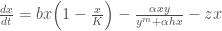

 is the prey population being harvested and
  is the predator population. Please refer to
 , rather than specific parameter values,
 ![z = [z_1, z_2, ..., z_t]](https://s0.wp.com/latex.php?latex=z+%3D+%5Bz_1%2C+z_2%2C+...%2C+z_t%5D&bg=ffffff&fg=444444&s=0&c=20201002) . The process of optimizing the parameters of a state-aware control rule is known as Direct Policy Search (DPS; Quinn et al, 2017).
. The process of optimizing the parameters of a state-aware control rule is known as Direct Policy Search (DPS; Quinn et al, 2017). , is mapped to the current prey population levels,
  by the function:
![z_{t+1} = \sum_{i=1}^n w_i \Big[exp\Big[-\Big(\frac{x_t-c_i}{b_i}\Big)^2\Big]\Big]](https://s0.wp.com/latex.php?latex=z_%7Bt%2B1%7D+%3D+%5Csum_%7Bi%3D1%7D%5En+w_i+%5CBig%5Bexp%5CBig%5B-%5CBig%28%5Cfrac%7Bx_t-c_i%7D%7Bb_i%7D%5CBig%29%5E2%5CBig%5D%5CBig%5D&bg=ffffff&fg=444444&s=0&c=20201002)
 and
and  are the center, radius, and weights of each RBF
  respectively. Additionally,
  is the number of RBFs used in the function; in this study we use
  RBFs. With two RBFs, there are a total of 6 parameters. Increasing the number of RBFs allows for more flexible function forms to be achieved. However, two RBFs have been shown to be sufficient for this problem.
![[c_1, b_1, w_1, c_2, b_2, w_2]](https://s0.wp.com/latex.php?latex=%5Bc_1%2C+b_1%2C+w_1%2C+c_2%2C+b_2%2C+w_2%5D&bg=ffffff&fg=444444&s=0&c=20201002) ), and the current prey population, to calculate the next year’s harvesting effort.
), and the current prey population, to calculate the next year’s harvesting effort. .
.![[c_1, b_1, w_1, c_2, b_2, w_2] = [0.2, 1.1, 0.41, 0.34,0.7, 0.59]](https://s0.wp.com/latex.php?latex=%5Bc_1%2C+b_1%2C+w_1%2C+c_2%2C+b_2%2C+w_2%5D+%3D+%5B0.2%2C+1.1%2C+0.41%2C+0.34%2C0.7%2C+0.59%5D+&bg=ffffff&fg=444444&s=0&c=20201002)

![c_i, b_i, w_i \in [0,1]](https://s0.wp.com/latex.php?latex=c_i%2C+b_i%2C+w_i+%5Cin+%5B0%2C1%5D&bg=ffffff&fg=444444&s=0&c=20201002) . Below is a plot of the resulting random policy functions:
. Below is a plot of the resulting random policy functions: times, and take the average objective score over the range of simulations. This method helps to account for variability in expected outcomes due to natural stochasticity. Here, we use
  realizations of stochasticity.
 ) is calculated as:
 is the discount rate which converts future benefits to present economic value, here
  .
. :
: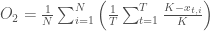


 .
.

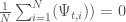


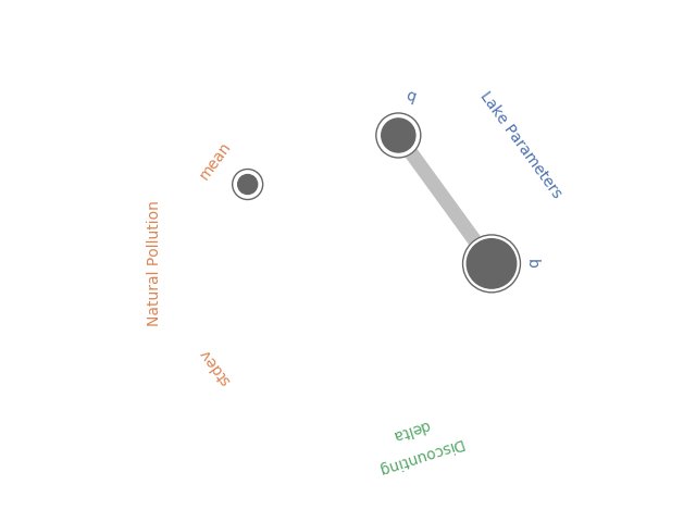


 ,
,  and
and  are the centers, radii and wights of n cubic radial basis functions. These parameters will be the decision variables for our multi-objective optimization (searching for parameters to a rule system like this is known as direct policy search (DPS)). For this example we’ll use n=2 cubic radial basis functions and have 6 decision variables.
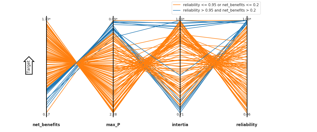
![R1 = \max_i[D_{i,90}:P(D_i\leq D_{i,90}=0.90]](https://s0.wp.com/latex.php?latex=R1+%3D+%5Cmax_i%5BD_%7Bi%2C90%7D%3AP%28D_i%5Cleq+D_%7Bi%2C90%7D%3D0.90%5D&bg=ffffff&fg=444444&s=0&c=20201002)
 represents the value of objective i in the baseline SOW and
  represents the value of objective i calculated in SOW j.
 ![R2 = \max_i[D_{i,90}:P(D_i\leq D_{i,90}=0.90]](https://s0.wp.com/latex.php?latex=R2+%3D+%5Cmax_i%5BD_%7Bi%2C90%7D%3AP%28D_i%5Cleq+D_%7Bi%2C90%7D%3D0.90%5D&bg=ffffff&fg=444444&s=0&c=20201002)


 = 1 if solution s meets the performance criteria in SOW j and
 ![S2 = \hat{\alpha} = max \big[\alpha:min_{j \in U(\alpha)} F(x)_j \geq r^* \big]](https://s0.wp.com/latex.php?latex=S2+%3D+%5Chat%7B%5Calpha%7D+%3D+max+%5Cbig%5B%5Calpha%3Amin_%7Bj+%5Cin+U%28%5Calpha%29%7D+F%28x%29_j+%5Cgeq+r%5E%2A+%5Cbig%5D&bg=ffffff&fg=444444&s=0&c=20201002)
 = maximum level of uncertainty, measured outward from the base SOW that can be tolerated before performance drops below threshold r*. In this example, I’ll normalize all uncertainties to their sampling range. In the function below, results is once again a Rhodium DataSet object containing the full set of DU reevaluations for one member of the Pareto approximate set. baseline is a DataSet containing the solution’s performance in the baseline state of the world. uncertainties_min is a list containing the lower bound for each uncertainty and uncertainties_max is a list containing upper bounds.
