In these posts, we explored the complex dynamics of a two-species predator-prey fisheries system. We also visualized various potential scenarios of stability and collapse that result from a variety of system parameter values. We then set up the problem components that include its parameters and their associated uncertainty ranges, performance objectives and the radial basis functions (RBFs) that map the current system state to policy action
Now, we will building off the previous posts and generate the full Pareto-approximate set of performance objectives and their associated decision variable values. We will also specify our robustness multivariate satisficing criteria (Starr, 1963) set by Hadjimichael et al (2020) and use J3, a visualization software, to explore the tradeoff space and identify the solutions that meet these criteria.
To better follow along with our training series, please find the accompanying GitHub repository that contains all the source code here.
A brief recap on decision variables, parameters and performance objectives
In the Fisheries Training series, we describe the system using the following parameters:
and : The prey and predator population densities at time respectively
: The rate at which the predator encounters the prey
: The prey growth rate
: The rate at which the predator converts prey to new predators
: The predator death rate
: The time the predator needs to consume the prey (handling time)
: Environmental carrying capacity
: The level of predator interaction
: The fraction of prey that is harvested
Please refer to Post 0 for further details on the relevance of each parameter.
Our decision variables are the three RBF parameters: the center (), radius () and weights () of each RBF respectively. From Part 1, we opt to use two RBFs where to result in six decision variables.
Next, our objectives are as follows:
Objective 1: Maximize net present value (NPV)
Objective 2: Minimize prey-population deficit
Objective 3: Minimize the longest duration of consecutive low harvest
Objective 4: Minimize worst harvest instance
Objective 5: Minimize harvest variance
Detailed explanation on the formulation and Python execution of the RBFs and objectives can be found in Post 1.
Now that we’ve reviewed the problem setup, let’s get to setting up the code!
Running the full problem optimization
Importing all libraries and setting up the problem
Before beginning, ensure that both Platypus and PyBorg are downloaded and installed as recommended by Post 1. Next, as previously performed, import all the necessary libraries:
# import all required libraries
from platypus import Problem, Real, Hypervolume, Generator
from pyborg import BorgMOEA
from fish_game_functions import *
from platypus import Problem, Real, Hypervolume, Generator
from pyborg import BorgMOEA
import matplotlib.pyplot as plt
import time
import random
We then define the problem by setting the number of variables (nVars), performance objectives (nObjs) and constraints (nCnstr). We also define the upper and lower bounds of each objective. The negative values associated with Objectives 1 and 4 indicate that they are to be maximized.
# Set the number of decision variables, constraints and performance objectives
nVars = 6   # Define number of decision variables
nObjs = 5   # Define number of objectives
nCnstr = 1      # Define number of decision constraints

# Define the upper and lower bounds of the performance objectives
objs_lower_bounds = [-6000, 0, 0, -250, 0]
objs_upper_bounds = [0, 1, 100, 0, 32000]
Then we initialize the algorithm (algorithm) to run over 10,000 function evaluations (nfe) with a starting population of 500 (pop_size):
# initialize the optimization
algorithm = fisheries_game_problem_setup(nVars, nObjs, nCnstr)
nfe = 10000    # number of function evaluations
pop_size = 500    # population size
Storing the Pareto-approximate objectives and decision variables
We are ready to run this (Fisheries) world! But first, we will open two CSV files where we will store the Pareto-approximate objectives (Fisheries2_objs.csv) and their associated decision variables (Fisheries2_vars.csv). These are the (approximately) optimal performance objective values and the RBF () vectors that give rise to them discovered by PyBorg. We also record the total amount of time it takes to optimize the Fisheries over 10,000 NFEs with a population of 500.
# open file in which to store optimization objectives and variables
f_objs = open('Fisheries2_objs.txt', "w+")
f_vars = open('Fisheries2_vars.txt', "w+")

# get number of algorithm variables and performance objectives
nvars = algorithm.problem.nvars
nobjs = algorithm.problem.nobjs

# begin timing the optimization
opt_start_time = time.time()

algorithm = fisheries_game_problem_setup(nVars, nObjs, nCnstr, pop_size=int(pop_size))
algorithm.run(int(nfe))

# get the solution archive
arch = algorithm.archive[:]
for i in range(len(arch)):
    sol = arch[i]
    # write objectives to file
    for j in range(nobjs):
        f_objs.write(str(sol.objectives[j]) + " ")
    # write variables to file
    for j in range(nvars):
        f_vars.write(str(sol.variables[j]) + " ")

    f.write("\n")

# end timing and print optimization time
opt_end_time = time.time()

opt_total_time = opt_end_time - opt_start_time

f_objs.close()
f_vars.close()

# print the total time to console
print(format"\nTime taken = ", {opt_total_time})
The optimization should take approximately 3,100 seconds or 52 minutes. When the optimization is completed, you should be able to locate the Fisheries2_objs.txt and Fisheries2_vars.txt files in the same folder where the Jupyter notebook is stored.
Post-Processing
To ensure that our output can be used in our following steps, we perform post-processing to convert the .txt files into .csv files.
import numpy as np

# convert txt files to csv
# load the .txt files as numpy matrices
matrix_objs = np.genfromtxt('Fisheries2_objs.txt', delimiter=' ')
matrix_vars = np.genfromtxt('Fisheries2_vars.txt', delimiter=' ')

# reshape the matrices
# the objectives file should have shape (n_solns, nObjs)
# the variables file should have shape (n_solns, nVars)
n_solns = int(matrix_objs.shape[0]/nObjs)

matrix_objs = np.reshape(matrix_objs, (n_solns,nObjs))
matrix_vars = np.reshape(matrix_vars, (n_solns,nVars))

# label the objectives and variables
objs_names = ['NPV', 'Pop_Deficit', 'Low_Harvest', 'Worst_Harvest', 'Variance']
var_names = ['c1', 'r1', 'w1', 'c2', 'r2', 'w2']

# Convert the matrices to dataframes with header names
df_objs = pd.DataFrame(matrix_objs, columns=objs_names)
df_vars = pd.DataFrame(matrix_vars, columns=var_names)

# save the processed matrices as csv files
df_objs.to_csv('Fisheries2_objs.csv', sep=',', index=False)
df_vars.to_csv('Fisheries2_vars.csv', sep=',', index=False)
You should now be able to locate the Fisheries2_objs.csv and Fisheries2_vars.csv within the same folder where you store the Jupyter Notebook.
In the following steps, we will introduce the J3 Visualization Software, which takes .csv files as inputs, to visualize and explore the tradeoff space of the fisheries problem.
Introduction to visualization with J3
J3 is an open-sourced app to produce and share high-dimensional, interactive scientific visualizations. It is part of the larger Project Platypus, which is a collection of libraries that aid in decision-making, optimization, and data visualization. It is influenced by D3.js, which is a JavaScript library for manipulating data using documents (data-driven documents; hence the name). Instead of documents, J3 manipulates data using many-dimensional plots, annotations and animations.
There is a prior post by Antonia Hadjimichael that covers the Python implementation of J3. In this post, we will be exploring the J3 app itself.
Installing and setting up J3
To use J3, you should first install Java. Please follow the directions found on the official Java site to select the appropriate installation package for your operating system.
Next, you can install J3 in either one of two ways:
Download the .zip file from the J3 Github Repository and extract its contents into a desired location on your location machine.
Install using git clone:
cd your-desired-location-path
git clone https://github.com/Project-Platypus/J3.git
You should now see a folder called ‘J3’ located in the path where you chose to extract the repository. Run the J3.exe file within the folder as shown below:
Next, we upload our Fisheries2_objs.csv file into J3:
The GIF below shows the a 3D tradeoff plot that is used to demonstrate the functions that each of the toggles serve. In this 3D plot, the NPV and Harvest Variance are seen on the x- and y-axes, while the Worst-case Harvest is seen on the z-axis. The size of the points represents Lowest Harvest Instance and their colors demonstrate the Population Size.
Other functions not shown above include:
Zooming in by scrolling on your mouse or trackpad
Deleting the annotations by right-clicking on them
Pressing the ‘esc’ key to de-select a point of interest
Next, we can also generate accompanying 2D-scatter and parallel axis plots to this 3D tradeoff figure:
In the parallel axis plot, the direction of preference is upwards. Here, we can visualize the significant tradeoffs between net present cost of the fisheries’ yield and population deficit. If stakeholders wish to maximize the economic value of the fisheries, they may experience unsustainable prey population deficits. The relationship between the remaining objectives is less clear. In J3, you can move the parallel axis plot axes to better visualize the tradeoffs between two objectives:
Here, we observe that there is an additional tradeoff between the minimizing the population deficit and maintaining low occurrences of low-harvest events. From this brief picture, we can observe that the main tradeoffs within the Fisheries system are between ecological objectives such as population deficit and economic objectives such as net present value and harvest.
Note the Brushing tool that appears next to the parallel axis plot. This will be important as we begin our next step, and that is defining our robustness multivariate satisficing criteria.
The multivariate satisficing criteria and identifying robust solutions
The multivariate satisficing criteria is derived from Starr’s domain criterion satisficing measure (Starr, 1962). In Hadjimichael et al. (2020), the multivariate satisficing criteria was selected as it allowed the identification of solutions that meet stakeholders’ competing requirements. In the context of Part 2, we use these criteria to identify the solutions in the Pareto-approximate set that satisfy the expectations of stakeholder. Here, the requirements are as follows:
Net present value (NPV) 1,500
Prey-population deficit 0.5
Longest duration of consecutive low harvest 5
Worst harvest instance 50
Harvest variance 1
Using the brushing tool to highlight only the solutions of interest, we find a pared-down version of the Pareto set. This tells us that not all optimal solutions are realistic, feasible, or satisfactory to decision-makers in the Fisheries system.
Conclusion
Good job with making it this far! Your accomplishments are many:
You ran a full optimization of the Fisheries Problem.
Your downloaded, installed, and learned how to use J3 to visualize and manipulate data to explore the tradeoff space of the Fisheries system.
You learned about Multivariate Satisficing Criteria to identify solution tradeoffs that are acceptable to the stakeholders within the Fisheries system.
In our next post, we will further expand on the concept of the multivariate satisficing criteria and use it to evaluate how 2-3 of the different solutions that were found to initially satisfy stakeholder requirements when tested across more challenging scenarios. But in the meantime, we recommend that you explore the use of J3 on alternative datasets as well, and see if you can come up with an interesting narrative based on your data!
Until then, happy visualizing!
References
Giuliani, M., Castelletti, A., Pianosi, F., Mason, E. and Reed, P., 2016. Curses, Tradeoffs, and Scalable Management: Advancing Evolutionary Multiobjective Direct Policy Search to Improve Water Reservoir Operations. Journal of Water Resources Planning and Management, 142(2).
Hadjimichael, A., Reed, P. and Quinn, J., 2020. Navigating Deeply Uncertain Tradeoffs in Harvested Predator-Prey Systems. Complexity, 2020, pp.1-18.
Starr, M., 1963. Product design and decision theory. Journal of the Franklin Institute, 276(1), p.79.
Welcome to the second post in the Fisheries Training Series, in which we are studying decision making under deep uncertainty within the context of a complex harvested predator-prey fishery. The accompanying GitHub repository, containing all of the source code used throughout this series, is available here. The full, in-depth Jupyter Notebook version of this post is available in the repository as well.
A brief re-cap of the harvested predator-prey model
Formulation of the harvesting policy and an overview of radial basis functions (RBFs)
Formulation of the policy objectives
A simulation model for the harvested system
Optimization of the harvesting policy using the PyBorg MOEA
Installation of Platypus and PyBorg*
Optimization problem formulation
Basic MOEA diagnostics
Note *The PyBorg MOEA used in this demonstration is derived from the Borg MOEA and may only be used with permission from its creators. Fortunately, it is freely available for academic and non-commercial use. Visit BorgMOEA.org to request access.
Now, onto the tutorial!
Harvested predator-prey model
In the previous post, we introduced a modified form of the Lotka-Volterra system of ordinary differential equations (ODEs) defining predator-prey population dynamics.
This modified version includes a non-linear predator population growth dynamic original proposed by Arditi and Akçakaya (1990), and includes a harvesting parameter, . This system of equations is defined in Hadjimichael et al. (2020) as:
Where is the prey population being harvested and is the predator population. Please refer to Post 0 of this series for the rest of the parameter descriptions, and for insights into the non-linear dynamics that result from these ODEs. It also demonstrates how the system alternates between ‘basins’ of stability and population collapse.
Harvesting policy
In this post, we instead focus on the generation of harvesting policies which can be operated safely in the system without causing population collapse. Rather than assigning a deterministic (specific, pre-defined) harvest effort level for every time period, we instead design an adaptive policy which is a function of the current state of the system:
The problem then becomes the optimization of the control rule, , rather than specific parameter values, . The process of optimizing the parameters of a state-aware control rule is known as Direct Policy Search (DPS; Quinn et al, 2017).
Previous work done by Quinn et al. (2017) showed that an adaptive policy, generated using DPS, was able to navigate deeply uncertain ecological tipping points more reliably than intertemporal policies which prescribed specific efforts at each timestep.
Radial basis functions
The core of the DPS method are radial basis functions (RBFs), which are flexible, parametric function formulations that map the current state of the system to policy action. A previous study by Giuliani et al (2015) demonstrated that RBFs are highly effective in generating Pareto-approximate sets of solutions, and that they perform well when applied to horizons different from the optimized simulation horizon.
There are various RBF approaches available, such as the cubic RBF used by Quinn et al. (2017). Here, we use the Gaussian RBF introduced by Hadjimichael et al. (2020), where the harvest effort during the next timestep, , is mapped to the current prey population levels, by the function:
In this formulation and are the center, radius, and weights of each RBF respectively. Additionally, is the number of RBFs used in the function; in this study we use RBFs. With two RBFs, there are a total of 6 parameters. Increasing the number of RBFs allows for more flexible function forms to be achieved. However, two RBFs have been shown to be sufficient for this problem.
The sum of the weights must be equal to one, such that:
The function harvest_streategy() is contained within the fish_game_functions.py script, which can be accessed here in the repository.
A simplified rendition of the harvest_strategy() function, evaluate_RBF(), is shown below and uses the RBF parameter values (i.e., ), and the current prey population, to calculate the next year’s harvesting effort.
import numpy as np
import matplotlib.pyplot as plt

def evaluate_RBF(x, RBF_params, nRBFs):
    """
    Parameters:
    -----------
    x : float
        The current state of the system.
    RBF_params : list [3xnRBFs]
        The RBF parameters in the order of [c, r, w,...,c, r, w].
    nRBFs : int
        The number of RBFs used in the mapping function.

    Returns:
    --------
    z : float
        The policy action.
    """

    c = RBF_params[0::3]
    r = RBF_params[1::3]
    w = RBF_params[2::3]

    # Normalize the weights
    w_norm = []
    if np.sum(w) != 0:
        for w_i in w:
            w_norm.append(w_i / np.sum(w))
    else:
        w_norm = (1/nRBFs)*np.ones(len(w))

    z = 0.0

    for i in range(nRBFs):

        # Avoid division by zero
        if r[i] != 0:
            z = z + w[i] * np.exp(-((x - c[i])/r[i])**2)
        else:
            z = z + w[i] * np.exp(-((x - c[i])/(10**-6))**2)

    # Impose limits on harvest effort
    if z < 0:
        z = 0
    elif z > 1:
        z = 1

    return z
To better understand the nature of the harvesting policy, it is helpful to visualize the policy function, .
For some arbitrary selection of RBF parameters:
The following function will plot the harvesting strategy:
def plot_RBF_policy(x_range, x_label, y_range, y_label, RBF_params, nRBFs):
    """
    Parameters:
    -----------
    RBF_params : list [3xnRBFs]
        The RBF parameters in the order of [c, r, w,...,c, r, w].
    nRBFs : int
        The number of RBFs used in the mapping function.

    Returns:
    --------
    None.
    """
    # Step size
    n = 100
    x_min = x_range[0]
    x_max = x_range[1]
    y_min = y_range[0]
    y_max = y_range[1]

    # Generate data
    x_vals = np.linspace(x_min, x_max, n)
    y_vals = np.zeros(n)

    for i in range(n):
        y = evaluate_RBF(x_vals[i], RBF_params, nRBFs)

        # Check that assigned actions are within range
        if y < y_min:
            y = y_min
        elif y > y_max:
            y = y_max

        y_vals[i] = y

    # Plot
    fig, ax = plt.subplots(figsize = (5,5), dpi = 100)
    ax.plot(x_vals, y_vals, label = 'Policy', color = 'green')
    ax.set_xlabel(x_label)
    ax.set_ylabel(y_label)
    ax.set_title('RBF Policy')
    plt.show()
    return
Let’s take a look at the policy that results from the random RBF parameters listed above. Setting my problem-specific inputs, and running the function:
This policy does not make much intuitive sense… why should harvesting efforts be decreased when the fish population is large? Well, that’s because we chose these RBF parameter values randomly.
To demonstrate the flexibility of the RBF functions and the variety of policy functions that can result from them, I generated a few (n = 7) policies using a random sample of parameter values. The parameter values were sampled from a uniform distribution over each parameters range: . Below is a plot of the resulting random policy functions:
Fig: Many random RBF policies, showing flexibility of RBFs.
Finding the sets of RBF parameter values that result in Pareto-optimal harvesting policies is the next step in this process!
Harvest strategy objectives
We take a multi-objective approach to the generation of a harvesting strategy. Given that the populations are vulnerable to collapse, it is important to consider ecological objectives in the problem formulation.
Here, we consider five objectives, described below.
Objective 1: Net present value
The net present value (NPV) is an economic objective corresponding to the amount of fish harvested.
During the simulation-optimization process (later in this post), we simulate a single policy times, and take the average objective score over the range of simulations. This method helps to account for variability in expected outcomes due to natural stochasticity. Here, we use realizations of stochasticity.
With that in mind, the NPV () is calculated as:
where is the discount rate which converts future benefits to present economic value, here .
Objective 2: Prey population deficit
The second objective aims to minimize the average prey population deficit, relative to the prey population carrying capacity, :
Objective 3: Longest duration of consecutive low harvest
In order to maintain steady harvesting levels, we minimize the longest duration of consecutive low harvests. Here, a subjective definition of low harvest is imposed. In a practical decision making process, this threshold may be solicited from the relevant stakeholders.
Objective 3 is defined as:
where
And the low harvest limit is: .
Objective 4: Worst harvest instance
In addition to avoiding long periods of continuously low harvest, the stakeholders have a desire to limit financial risks associated with very low harvests. Here, we minimize the worst 1% of harvest.
The fourth objective is defined as:
Objective 5: Harvest variance
Lastly, policies which result in low harvest variance are more easily implemented, and can limit corresponding variance in fish populations.
The last objective minimizes the harvest variance, with the objective score defined as:
Constraint: Avoid collapse of predator population
During the optimization process, we are able to include constraints on the harvesting policies.
Since population collapse is a stable equilibrium point, from which the population will not regrow, it is imperative to consider policies which prevent collapse.
With this in mind, the policy must not result in any population collapse across the realizations of environmental stochasticity. Mathematically, this is enforced by:
where
Problem formulation
Given the objectives described above, the optimization problem is:
Simulation model of the harvested system
Here, we provide an overview of the fish_game_5_objs() model which combines many of the preceding topics. The goal for this model is to take a set of RBF parameters, which define the harvesting strategy, simulate the policy for some length of time, and then return the objective scores resulting from the policy.
Later, this model will allow for the optimization of the harvesting policy RBF parameters through a Multi-Objective Evolutionary Algorithm (MOEA). The MOEA will evaluate many thousands of policies (RBF parameter combinations) and attempt to find, through evolution, those RBF parameters which yield best objective performance.
A brief summary of the model process is described here, but the curious learner is encouraged to take a deeper look at the code and dissect the process.
The model can be understood as having three major sections:
Initialization of storage vectors, stochastic variables, and assumed ODE parameters.
Simulation of policy and fishery populations over time period T.
Calculation of objective scores.
def fish_game_5_objs(vars):
    """
    Defines the full, 5-objective fish game problem to be solved

    Parameters
    ----------
    vars : list of floats
        Contains the C, R, W values

    Returns
    -------
    objs, cnstr
    """

    # Get chosen strategy
    strategy = 'Previous_Prey'

    # Define variables for RBFs
    nIn = 1 # no. of inputs (depending on selected strategy)
    nOut = 1 # no. of outputs (depending on selected strategy)
    nRBF = 2 # no. of RBFs to use

    nObjs = 5
    nCnstr = 1 # no. of constraints in output

    tSteps = 100 # no. of timesteps to run the fish game on
    N = 100 # Number of realizations of environmental stochasticity

    # Define assumed system parameters
    a = 0.005
    b = 0.5
    c = 0.5
    d = 0.1
    h = 0.1
    K = 2000
    m = 0.7
    sigmaX = 0.004
    sigmaY = 0.004

    # Initialize storage arrays for populations and harvest
    x = np.zeros(tSteps+1) # Prey population
    y = np.zeros(tSteps+1) # Predator population
    z = np.zeros(tSteps+1) # Harvest effort

    # Create array to store harvest for all realizations
    harvest = np.zeros([N,tSteps+1])
    # Create array to store effort for all realizations
    effort = np.zeros([N,tSteps+1])
    # Create array to store prey for all realizations
    prey = np.zeros([N,tSteps+1])
    # Create array to store predator for all realizations
    predator = np.zeros([N,tSteps+1])

    # Create array to store metrics per realization
    NPV = np.zeros(N)
    cons_low_harv = np.zeros(N)
    harv_1st_pc = np.zeros(N)
    variance = np.zeros(N)

    # Create arrays to store objectives and constraints
    objs = [0.0]*nObjs
    cnstr = [0.0]*nCnstr

    # Create array with environmental stochasticity for prey
    epsilon_prey = np.random.normal(0.0, sigmaX, N)

    # Create array with environmental stochasticity for predator
    epsilon_predator = np.random.normal(0.0, sigmaY, N)

    # Go through N possible realizations
    for i in range(N):

        # Initialize populations and values
        x[0] = prey[i,0] = K
        y[0] = predator[i,0] = 250
        z[0] = effort[i,0] = harvest_strategy([x[0]], vars, [[0, K]], [[0, 1]], nIn, nOut, nRBF)
        NPVharvest = harvest[i,0] = effort[i,0]*x[0]

        # Go through all timesteps for prey, predator, and harvest
        for t in range(tSteps):

            # Solve discretized form of ODE at subsequent time step
            if x[t] > 0 and y[t] > 0:
                x[t+1] = (x[t] + b*x[t]*(1-x[t]/K) - (a*x[t]*y[t])/(np.power(y[t],m)+a*h*x[t]) - z[t]*x[t])* np.exp(epsilon_prey[i]) # Prey growth equation
                y[t+1] = (y[t] + c*a*x[t]*y[t]/(np.power(y[t],m)+a*h*x[t]) - d*y[t]) *np.exp(epsilon_predator[i]) # Predator growth equation

                # Solve for harvesting effort at next timestep
                if t <= tSteps-1:
                    if strategy == 'Previous_Prey':
                        input_ranges = [[0, K]] # Prey pop. range to use for normalization
                        output_ranges = [[0, 1]] # Range to de-normalize harvest to
                        z[t+1] = harvest_strategy([x[t]], vars, input_ranges, output_ranges, nIn, nOut, nRBF)

            # Store values in arrays
            prey[i,t+1] = x[t+1]
            predator[i,t+1] = y[t+1]
            effort[i,t+1] = z[t+1]
            harvest[i,t+1] = z[t+1]*x[t+1]
            NPVharvest = NPVharvest + harvest[i,t+1]*(1+0.05)**(-(t+1))

        # Solve for objectives and constraint
        NPV[i] = NPVharvest
        low_hrv = [harvest[i,j]<prey[i,j]/20 for j in range(len(harvest[i,:]))] # Returns a list of True values when there's harvest below 5%
        count = [ sum( 1 for _ in group ) for key, group in itertools.groupby( low_hrv ) if key ] # Counts groups of True values in a row
        if count: # Checks if theres at least one count (if not, np.max won't work on empty list)
            cons_low_harv[i] = np.max(count)  # Finds the largest number of consecutive low harvests
        else:
            cons_low_harv[i] = 0
        harv_1st_pc[i] = np.percentile(harvest[i,:],1)
        variance[i] = np.var(harvest[i,:])

    # Average objectives across N realizations
    objs[0] = -np.mean(NPV) # Mean NPV for all realizations
    objs[1] = np.mean((K-prey)/K) # Mean prey deficit
    objs[2] = np.mean(cons_low_harv) # Mean worst case of consecutive low harvest across realizations
    objs[3] = -np.mean(harv_1st_pc) # Mean 1st percentile of all harvests
    objs[4] = np.mean(variance) # Mean variance of harvest

    cnstr[0] = np.mean((predator < 1).sum(axis=1)) # Mean number of predator extinction days per realization

    # output should be all the objectives, and constraint
    return objs, cnstr
The next section shows how to optimize the harvest policy defined by vars, using the PyBorg MOEA.
A (Very) Brief Overview of PyBorg
PyBorg is the secondary implementation of the Borg MOEA written entirely in Python by David Hadka and Andrew Dircks. It is made possible using functions from the Platypus optimization library, which is a Python evolutionary computing framework.
As PyBorg is Borg’s Python wrapper and thus derived from the original Borg MOEA, it can only be used with permission from its creators. To obtain permission for download, please visit BorgMOEA and complete the web form. You should receive an email with the link to the BitBucket repository shortly.
Installation
The repository you have access to should be named ‘Serial Borg MOEA’ and contain a number of folders, including one called Python/. Within the Python/ folder, you will be able to locate a folder called pyborg. Once you have identified the folder, please follow these next steps carefully:
Check your current Python version. Python 3.5 or later is required to enable PyBorg implementation.
Download the pyborg folder and place it in the folder where this Jupyter Notebook all other Part 1 training material is located.
Install the platypus library. This can be in done via your command line by running one of two options:
Make sure the following training startup files are located within the same folder as this Jupyter Notebook: a) fish_game_functions.py: Contains all function definitions to setup the problem, run the optimization, plot the hypervolume, and conduct random seed analysis. b) Part 1 - Harvest Optimization and MOEA Diagnostics.ipynb: This is the current notebook and where the Fisheries fame will be demonstrated.
We are now ready to proceed!
Optimization of the Fisheries Game
Import all libraries
All functions required for this post can be found in the fish_game_functions.py file. This code is adapted from Antonia Hadjimichael’s original post on exploring the Fisheries Game dynamics using PyBorg.
# import all required libraries
from platypus import Problem, Real, Hypervolume, Generator
from pyborg import BorgMOEA
from fish_game_functions import *
from platypus import Problem, Real, Hypervolume, Generator
from pyborg import BorgMOEA
import time
import random
Formulating the problem
Define number of decision variables, constraints, and specify problem formulation:
# Set the number of decision variables, constraints and performance objectives
nVars = 6   # Define number of decision variables
nObjs = 5   # Define number of objectives
nCnstr = 1      # Define number of decision constraints

# Define the upper and lower bounds of the performance objectives
objs_lower_bounds = [-6000, 0, 0, -250, 0]
objs_upper_bounds = [0, 1, 100, 0, 32000]
Initialize the problem for optimization
We call the fisheries_game_problem_setup.py function to set up the optimization problem. This function returns a PyBorg object called algorithm in this exercise that will be optimized in the next step.
def fisheries_game_problem_setup(nVars, nObjs, nCnstr, pop_size=100):
    """
    Sets up and runs the fisheries game for a given population size

    Parameters
    ----------
    nVars : int
        Number of decision variables.
    nObjs : int
        Number of performance objectives.
    nCnstr : int
        Number of constraints.
    pop_size : int, optional
        Initial population size of the randomly-generated set of solutions.
        The default is 100.

    Returns
    -------
    algorithm : pyBorg object
        The algorthm to optimize with a unique initial population size.

    """
    # Set up the problem
    problem = Problem(nVars, nObjs, nCnstr)
    nVars = 6   # Define number of decision variables
    nObjs = 5   # Define number of objective -- USER DEFINED
    nCnstr = 1      # Define number of decision constraints

    problem = Problem(nVars, nObjs, nCnstr)

    # set bounds for each decision variable
    problem.types[0] = Real(0.0, 1.0)
    problem.types[1] = Real(0.0, 1.0)
    problem.types[2] = Real(0.0, 1.0)
    problem.types[3] = Real(0.0, 1.0)
    problem.types[4] = Real(0.0, 1.0)
    problem.types[5] = Real(0.0, 1.0)

    # all values should be nonzero
    problem.constraints[:] = "==0"

    # set problem function
    if nObjs == 5:
        problem.function = fish_game_5_objs
    else:
        problem.function = fish_game_3_objs

    algorithm = BorgMOEA(problem, epsilons=0.001, population_size=pop_size)
    return algorithm
# initialize the optimization
algorithm = fisheries_game_problem_setup(nVars, nObjs, nCnstr)
Define parameters for optimization
Before optimizing, we have to define our desired population size and number of function evaluations (NFEs). The NFEs correspond to the number of evolutions of the set of solutions. For complex, many-objective problems, it may be necessary for a large NFE.
Here, we start with a small limit on NFE, to test the speed of the optimization. Limiting the optimization to 100 NFE is going to produce relatively poor performing solutions, however it is a good starting point for our diagnostic tests.
init_nfe = 100
init_pop_size = 100
Begin the optimization
In addition to running the optimization, we also time the optimization to get a general estimate on the time the full hypervolume analysis will require.
# begin timing the Borg run
borg_start_time = time.time()

algorithm = fisheries_game_problem_setup(nVars, nObjs, nCnstr, pop_size=int(init_pop_size))
algorithm.run(int(init_nfe))

# end timing and print optimization time
borg_end_time = time.time()

borg_total_time = borg_end_time - borg_start_time

print(f"borg_total_time={borg_total_time}s")
Output: borg_total_time=33.62936472892761s
NOTICE: Running the PyBrog MOEA 100 times took ~34 seconds (on the machine which this was written on…). Keep this in mind, that increasing the NFE will require correspondingly more time. If you increase the number too much, your machine may take a long time to compute the final Pareto-front.
Plot the tradeoff surface
Here, we plot a 3-dimensional plot showing the tradeoff between a select number of objectives. If you have selected the 5-objective problem formulation, you should select the three objectives you would like to analyze the tradeoff surface for. Please select the (abbreviated) objective names from the following list:
Objective 1: Mean NPV Objective 2: Mean prey deficit Objective 3: Mean WCLH Objective 4: Mean 1% harvest Objective 5: Mean harvest variance
# Plot objective tradeoff surface
fig_objs = plt.figure(figsize=(8,8))
ax_objs = fig_objs.add_subplot(111, projection='3d')

# Select the objectives to plot from the list provided in the description above
obj1 = 'Mean NPV'
obj2 = 'Mean prey deficit'
obj3 = 'Mean 1% harvest'

plot_3d_tradeoff(algorithm, ax_objs, nObjs, obj1, obj2, obj3)
Fig: Pareto-approximate solutions generated with 100 function evaluations. The star is an ideal solution.
The objectives scores arn’t very good, but that is because the number of function evaluations is so low. In order to get a better set of solutions, we need to run the MOEA for many function evaluations.
The next section demonstrates the change in objective performance with respect to the number of function evaluations.
MOEA Diagnostics
A good MOEA is assessed by it’s ability to quickly converge to a set of solutions (the Pareto-approximate set) that is also diverse. This means that the final set of solutions is close to the true set, as well as covers a large volume of the multi-dimensional problem space. There are three quantitative metrics via which convergence and diversity are evaluated:
Generational distance approximates the average distance between the true Pareto front and the Pareto-approximate reference set that your MOEA identifies. It is the easiest metric to meet.
Epsilon indicator is a harder metric than generational distance to me et. A high-performing MOEA will have a low epsilon indicator value when the distance of its worst-performing approximate solution from the true Pareto set is small.
Hypervolume measures the ‘volume’ that a Pareto front covers across all dimensions of a problem. It is the hardest metric to meet and the most computationally intensive.
Both the generational distance and epsilon indicator metrics require a reference set, which is the known, true Pareto front. Conversely, the hypervolume does not have such a requirement. Given that the Fisheries Game is a complex, multi-dimensional, many-stakeholder problem with no known solution, the hypervolume metric is thus the most suitable to evaluate the ability of PyBorg to quickly converge to a diverse Pareto-approximate set of solutions.
The hypervolume is a measure of the multi-dimensional volume dominated by the approximated Pareto front. As the Pareto front advances toward the “ideal” solution, this value approaches 1.
The efficiency of an MOEA in optimizing a solution can be considered by measuring the hypervolume with respect to the number of function evaluations. This allows the user to understand how quickly the MOEA is converging to a good set of solutions, and how many function evaluations are needed to achieve a good set of solutions.
Defining hypervolume parameters
First, we define the maximum number of function evaluations (maxevals) and the NFE step size (frequency) for which we would like to evaluate the problem hypervolume over. Try modifying these values to see how the plot changes.
Mind that the value of maxevals should always be more than that of your initial NFE, and that the value of frequency should be less than that of the initial NFE. Both values should be integer values.
Also be mindful that increasing the maxevals > 1000 is going to result in long runtimes.
maxevals = 500
frequency = 100
Plotting the hypervolume
Using these parameters, we then plot the hypervolume graph, showing the change in hypervolume value over the NFEs.
Generally, RSA is performed to track an algorithm’s performance during search. In addition, it is also done to determine if an algorithm has discovered an acceptable approximation of the true Pareto set. More details on RSA can be found here in a blog post by Dave Gold.
For the Fisheries Game, we conduct RSA to determine if PyBorg’s performance is sensitive to the size of its initial population. We do this using the folllowing steps:
Run an ensemble of searches, each starting with a randomly sampled set of initial conditions (aka “random seeds”)
Combine search results across all random seeds to generate a “reference set” that contains only the best non-dominated solutions across the ensemble
Repeat steps 1 and 2 for an initial population size of 200, 400, etc.
pop_size_list = [100, 200, 400, 800, 1000]

fig_rand_seed = plt.figure(figsize=(10,7))
ax_rand_seed = fig_rand_seed.add_subplot()

for p in range(len(pop_size_list)):
    fisheries_game_problem_setup(nVars, nObjs, nCnstr, pop_size_list[p])
    algorithm = fisheries_game_problem_setup(nVars, nObjs, nCnstr, pop_size=int(init_pop_size))
    algorithm.run(int(init_nfe))

    plot_hvol(algorithm, maxevals, frequency, objs_lower_bounds, objs_upper_bounds,
              ax_rand_seed, pop_size_list[p])

plt.title('PyBorg Random Seed Analysis')
plt.xlabel('Number of Function Evaluations')
plt.ylabel('Hypervolume')
plt.legend()
plt.show()
Notice that the runs performed with different initial population sizes tend to converge toward a similar hypervolume value after 500 NFEs.
This reveals that the PyBorg MOEA is not very sensitive to the specific initial parameters; it is adaptable enough to succeed under different configurations.
Conclusion
A classic decision-making idiom says ‘defining the problem is the problem’. Hopefully, this post has revealed that to be true; we have shown that changes to the harvesting strategy functions, simulation model, or objective scores can result in changes to the resulting outcomes.
And if you’ve made it this far, congratulations! Take a minute to think back on the progression of this post: we revisited the harvested predator-prey model, formulated the harvesting policy using RBFs, and formulated the policy objectives and its associated simulation model. Next, we optimized the harvesting policy using the PyBorg MOEA and performed basic MOEA diagnostics using hypervolume as our measure, and executed random seed analysis.
If you’ve progressed through this tutorial using the Jupyter Notebook, we encourage you to re-visit the source code involved in this process. The next advisable step is to re-produce this problem from scratch, as this is the best way to develop a detailed understanding of the process.
Next time, we will explore the outcomes of this optimization, by considering the tradeoffs present across the Pareto set of solutions.
Simulation-optimization is an increasingly popular tool in many engineering fields. As the name implies, simulation-optimization requires two major components: a simulation model of the system we want to optimize (e.g., a water supply system) and an algorithm for iteratively tuning the decision levers within the system to optimize the simulated performance. For example, Multi-Objective Evolutionary Algorithms (MOEAs), such as the Borg MOEA, have been successfully employed across a variety of challenging stochastic multi-objective simulation-optimization problems in water resources and other fields. However, simulation-optimization can require millions of iterative simulation trials in order to adequately explore the decision and uncertainty spaces, especially under multi-objective framings. Given the ever-increasing size and complexity of simulation models, this can become a significant computational challenge.
Running the MOEA in parallel on high-performance computing clusters can greatly alleviate this challenge, but not eliminate it. For example, in my last blog post on hybrid parallelization of the Borg MOEA, I gave the example of optimizing infrastructure investments using a simulation model that takes 10 minutes to run a 30-year realization. Let’s assume we run 48 Monte Carlo realizations per function evaluation (FE) to account for natural hydrologic variability. Even using the maximum job size of 128 nodes on the Stampede2 supercomputer, with 48 CPU each, we will only be about to complete ~20,000 FEs per 24 hours of wall clock. To complete 100,000 FE, a relatively low target compared to other similarly-complex studies, the MOEA will need to run for ~5 days. This raises a major problem: many computing clusters have strict wall clock limits. On Stampede2, for example, each submission can run for a maximum of 48 hours. As a result, we would be limited to ~40,000 FE for a single Stampede2 run, which may be insufficient based on the difficulty of the problem.
Fortunately, the Borg MOEA’s “checkpointing” and “restoring” functionalities allow us to circumvent this issue. Checkpointing is the process of saving “snapshots” of the MOEA’s internal state at regular intervals, and restoring is the act of reading a snapshot into memory at the beginning of a run and continuing the optimization from that starting point. This allows us to effectively split a 5-day optimization into three sequential submissions, in order to comply with a 2-day wall clock limit. This functionality can also be helpful for iteratively assessing convergence, since we don’t necessarily know a priori how many FE will need to be run.
In this blog post, I will demonstrate the use of checkpointing and restoring with the Borg MOEA using a less computationally-demanding example: the Python-based DPS Lake Problem. However, the methods and results described here should be applicable to much larger experiments such as the one described above. See my last blog post and references therein for more details on the Python implementation of the DPS Lake Problem.
Setup
For this post, I ran the following short proof of concept: first I ran five random seeds of the Borg MOEA for 5 minutes each. Each seed was assigned 2 nodes (16 CPU each) on the Cube cluster at Cornell. Each seed completed approximately 6100 FE in this first round. Next, I ran a second round in which each seed began from the 6100-FE checkpoint and ran for another 5 minutes. All code for this post, along with instructions for downloading the correct branch of the Borg MOEA, can be found in this GitHub repository.
Setting up checkpointing only takes a few extra lines of code in the file “borg_lake_msmp.py”. First, we need to define the baseline file name used to store the checkpoint files:
Within the simulation, checkpoints will be made at regular intervals. The checkpoint file names will automatically have the FE appended; for example, the checkpoint for seed 5 after 6100 FE is written to “results/checkpoints/seed5_nfe6100.checkpoint”. The write frequency for both checkpoints and runtime metrics can be changed based on the “runtimeFrequency” parameter in “submit_msmp.sh”.
We can also provide a previous checkpoint to read in at the beginning of the run:
where “maxEvalsPrevious” is the number of FE for the prior checkpoint that we want to read in. This parameter is input in “submit_msmp.sh”. The previous checkpoint file must be placed in the “checkpoints” folder prior to runtime.
We provide both checkpoint file names to the Borg MOEA, along with other important parameters such as the maximum number of evaluations.
result = borg.solveMPI(maxEvaluations=maxEvals, runtime=runtimeFile, frequency=runtimeFreq, newCheckpointFileBase=newCheckpointFileBase, oldCheckpointFile=oldCheckpointFile, evaluationFile=evaluationFile)
The Python wrapper for the Borg MOEA will use this command to initialize and run the MOEA across all available nodes. For more details on the implementation of the experiment, see the GitHub repository above.
The checkpoint file
So what information is saved in the checkpoint file? This file includes all internal state variables needed to initialize a new instance of the Borg MOEA that begins where the previous run left off. As an example, I will highlight select information from “seed5_nfe6100.checkpoint”, the last checkpoint file (at 6100 FE) for seed 5 after the first round.
First, the file lists basic problem formulation information such as the number of objectives, the decision variable bounds, and the epsilon dominance parameters:
Version: 108000
Number of Variables: 6
Number of Objectives: 4
Number of Constraints: 1
Lower Bounds: -2 0 0 -2 0 0
Upper Bounds: 2 2 1 2 2 1
Epsilons: 0.01 0.01 0.0001 0.0001
Number of Operators: 6
Next, it lists current values for several parameters which evolve over the course of the optimization, such as the selection probabilities for the six recombination operators, the number of times the algorithm has triggered a “restart” due to stalled progress, and the number of solutions in the population:
Operator Selection Probabilities: 0.93103448275862066 0.0086206896551724137 0.017241379310344827 0.025862068965517241 0.0086206896551724137 0.0086206896551724137
Number of Evaluations: 6100
Tournament Size: 3
Window Size: 200
...
Number of Restarts: 0
...
Population Size: 196
Population Capacity: 196
The file then lists each of the 196 solutions currently stored in the population:
Each line in this section represents a different solution; the numbers represent the 6 decision variables, 4 objectives, and 1 constraints for this problem, as well as the index of the operator used to create each solution.
Similarly, the file lists the current archive, which is the subset of 64 solutions from the larger population that are non-dominated:
We see that after 6100 FE, the algorithm is almost exclusively using the operator with index 0; this is consistent with operator 0’s 93% selection probability listed earlier in the file.
Finally, the checkpoint file closes with the current state of the random number generator:
RNG State Length: 624
RNG State: 2103772999 2815404811 3893540187 ...
RNG Index: 200
Next Gaussian: -0.13978937466755278
Have Next Gaussian: 0
Results
So does it work? Figure 1 shows the convergence of the five seeds according to six different measures of quality for the evolving archive. Performance for all seeds is found to be continuous across the two rounds, suggesting that the checkpointing and restoring is working properly. Additionally, Figure 2 demonstrates the continuity of the auto-adaptive selection probabilities for the Borg MOEA’s different recombination operators.
Figure 1: Performance of 5 random seeds across 2 rounds, quantified by six different measures of approximate Pareto set quality.Figure 2: Adaptive selection probabilities for the Borg MOEA’s six recombination operators.
The checkpointing process thus allows for continuity of learning across rounds: not only learning about which solutions are most successful (i.e., continuity of the population and archive), but also learning about which strategies for generating new candidate solutions are most successful (i.e., continuity of the recombination operator histories and probabilities). This capability allows for seamlessly sequencing separate “blocks” of function evaluations in situations where wall clock limits are limiting, or where the convergence behavior of the problem is not well understood a priori.
PyBorg is a new secondary implementation of Borg, written entirely in Python using the Platypus optimization library. PyBorg was developed by Andrew Dircks based on the original implementation in C and it is intended primarily as a learning tool as it is less efficient than the original C version (which you can still use with Python but through the use of the plugin “wrapper” also found in the package). PyBorg can be found in the same repository where the original Borg can be downloaded, for which you can request access here: http://borgmoea.org/#contact
This blogpost is intended to demonstrate this new implementation. To follow along, first you need to either clone or download the BitBucket repository after you gain access.
Setting up the required packages is easy. In your terminal, navigate to the Python directory in the repository and install all prerequisites using python setup.py install. This will install all requirements (i.e. the Platypus library, numpy, scipy and six) for you in your current environment.
You can test that everything works fine by running the optimization on the DTLZ2 test function, found in dtlz2.py. The script creates an instance of the problem (as it is already defined in the Platypus library), sets it up as a ploblem for Borg to optimize and runs the algorithm for 10,000 function evaluations:
    # define a DTLZ2 problem instance from the Platypus library
    nobjs = 3
    problem = DTLZ2(nobjs)

    # define and run the Borg algorithm for 10000 evaluations
    algorithm = BorgMOEA(problem, epsilons=0.1)
    algorithm.run(10000)
A handy 3D scatter plot is also generated to show the optimization results.
The repository also comes with two other scripts dtlz2_runtime.py and dtlz2_advanced.py. The first demonstrates how to use the Platypus hypervolume indicator at a specified runtime frequency to get learn about its progress as the algorithm goes through function evaluations:
The latter provides more advanced functionality that allows you define custom parameters for Borg. It also includes a function to generate runtime data from the run. Both scripts are useful to diagnose how your algorithm is performing on any given problem.
The rest of this post is a demo of how you can use PyBorg with your own Python model and all of the above. I’ll be using a model I’ve used before, which can be found here, and I’ll formulate it so it only uses the first three objectives for the purposes of demonstration.
The first thing you need to do to optimize your problem is to define it. This is done very simply in the exact same way you’d do it on Project Platypus, using the Problem class:
from fishery import fish_game
from platypus import Problem, Real
from pyborg import BorgMOEA

# define a problem
nVars = 6
nObjs = 3

problem = Problem(nVars, nObjs) # first input is no of decision variables, second input is no of objectives
problem.types[:] = Real(0, 1) #defines the type and bounds of each decision variable
problem.function = fish_game #defines the model function
This assumes that all decision variables are of the same type and range, but you can also define them individually using, e.g., problem.types[0].
Then you define the problem for the algorithm and set the number of function evaluations:
algorithm = BorgMOEA(problem, epsilons=0.001) #epsilons for each objective
algorithm.run(10000) # number of function evaluations
If you’d like to also produce a runtime file you can use the detailed_run function included in the demo (in the files referenced above), which wraps the algorithm and runs it in intervals so the progress can be monitored. You can combine it with runtime_hypervolume to also track your hypervolume indicator. To use it you need to define the total number of function evaluations, the frequency with which you’d like the progress to be monitored and the name of the output file. If you’d like to calculate the Hypervolume (you first need to import it from platypus) you also need to either provide a known reference set or define maximum and minimum values for your solutions.
My full script can be found below. The detailed_run function is an edited version of the default that comes in the demo to also include the hypervolume calculation.
from fishery import fish_game
from platypus import Problem, Real, Hypervolume
from pyborg import BorgMOEA
from runtime_diagnostics import detailed_run
# define a problem
nVars = 6 # no. of decision variables to be optimized
nObjs = 3
problem = Problem(nVars, nObjs) # first input is no of decision variables, second input is no of objectives
problem.types[:] = Real(0, 1)
problem.function = fish_game
# define and run the Borg algorithm for 10000 evaluations
algorithm = BorgMOEA(problem, epsilons=0.001)
#algorithm.run(10000)
# define detailed_run parameters
maxevals = 10000
frequency = 100
output = "fishery.data"
hv = Hypervolume(minimum=[-6000, 0, 0], maximum=[0, 1, 100])

nfe, hyp = detailed_run(algorithm, maxevals, frequency, output, hv)
# plot the results using matplotlib
import matplotlib.pyplot as plt
from mpl_toolkits.mplot3d import Axes3D
fig = plt.figure()
ax = fig.add_subplot(111, projection='3d')
ax.scatter([s.objectives[0] for s in algorithm.result],
[s.objectives[1] for s in algorithm.result],
[s.objectives[2] for s in algorithm.result])
ax.set_xlabel('Objective 1')
ax.set_ylabel('Objective 2')
ax.set_zlabel('Objective 3')
ax.scatter(-6000, 0, 0, marker="*", c='orange', s=50)
plt.show()
plt.plot(nfe, hyp)
plt.title('PyBorg Runtime Hypervolume Fish game')
plt.xlabel('Number of Function Evaluations')
plt.ylabel('Hypervolume')
plt.show()
In most applications, parallel computing is used to improve code efficiency and expand the scope of problems that can be addressed computationally (for background on parallelization, see references listed at the bottom of this post). For the Borg Many Objective Evolutionary Algorithm (MOEA) however, parallelization can also improve the quality and reliability of many objective search by enabling a multi-population search. The multi-population implementation of Borg is known as Multi-Master Borg, details can be found here. To measure the performance of Multi-Master Borg, we need to go beyond basic parallel efficiency (discussed in my last post, here), which measures the efficiency of computation but not the quality of the many objective search. In this post, I’ll discuss how we measure the performance of Multi-Master Borg using two metrics: hypervolume speedup and reliability.
Hypervolume speedup
In my last post, I discussed traditional parallel efficiency, which measures the improvement in speed and efficiency that can be achieved through parallelization. For many objective search, speed and efficiency of computation are important, but we are more interested in the speed and efficiency with which the algorithm produces high quality solutions. We often use the hypervolume metric to measure the quality of an approximation set as it captures both convergence and diversity (for a thorough explanation of hypervolume, see this post). Using hypervolume as a measure of search quality, we can then evaluate hypervolume speedup, defined as:
Hypervolume speedup =
where is the time it takes the serial version of the MOEA to achieve a given hypervolume threshold, and is the time it takes the parallel implementation to reach the same threshold. Figure 1 below, adapted from Hadka and Reed, (2014), shows the hypervolume speedup across different parallel implementations of the Borg MOEA for the five objective NSGA II test problem run on 16,384 processors (in this work the parallel epsilon-NSGA II algorithm is used as a baseline rather than a serial implementation). Results from Figure 1 reveal that the Multi-Master implementations of Borg are able to reach each hypervolume threshold faster than the baseline algorithm and the master-worker implementation. For high hypervolume thresholds, the 16 and 32 Master implementations achieve the hypervolume thresholds 10 times faster than the baseline.
Figure 1: Hypervolume speedup for the five objective LRGV test problem across implementations of the Borg MOEA (epsilon NSGA-II, another algorithm) is used as the baseline here). This figure is adapted from Hadka and Reed, (2014).
Reliability
MOEAs are inherently stochastic algorithms, they are be initialized with random seeds which may speedup or slow down the efficiency of the search process. To ensure high quality Pareto approximate sets, it’s standard practice to run an MOEA across many random seeds and extract the best solutions across all seeds as the final solution set. Reliability is a measure of the probability that each seed will achieve a high quality set of solutions. Algorithms that have higher reliability allow users to run fewer random seeds which saves computational resources and speeds up the search process. Salazar et al., (2017) examined the performance of 17 configurations of Borg on the Lower Susquehanna River Basin (LSRB) for a fixed 10 hour runtime. Figure 2 shows the performance of each configuration across 50 random seeds. A configuration that is able to achieve the best hypervolume across all seeds would be represented as a blue bar that extends to the top of the plot. The algorithmic configurations are shown in the plot to the right. These results show that though configuration D, which has a high core count and low master count, achieves the best overall hypervolume, it does not do so reliably. Configuration H, which has two masters, is able to achieve nearly the same hypervolume, but has a much higher reliability. Configuration L, which has four masters, achieves a lower maximum hypervolume, but has vary little variance across random seeds.
Figure 2: Reliability of search adapted from Salazar et al., (2017). Each letter represents a different algorithmic configuration (shown right) for the many objective LSRB problem across 10 hours of runtime. The color represents the probability that each configuration was able to attain a given level of hypervolume across 50 seeds.
These results can be further examined by looking at the quality of search across its runtime. In Figure 3, Salazar et al. (2017) compare the performance of the three algorithmic configurations highlighted above (D, H and L). The hypervolume achieved by the maximum and minimum seeds are shown in the shaded areas, and the median hypervolume is shown with each line. Figure 3 clearly demonstrates how improved reliability can enhance search. Though the Multi-Master implementation is able to perform fewer function evaluations in the 10 hour runtime, it has very low variance across seeds. The Master-worker implementation on the other hand achieves better performance with it’s best seed (it gets lucky), but its median performance never achieves the hypervolume of the two or four master configurations.
Figure 3: Runtime hypervolume dynamics for the LSRB problem by Salazar et al., (2017). The reduction in variance in the Multi-Master implementations of Borg demonstrate the benefits of improved reliability.
Concluding thoughts
The two measures introduced above allow us to quantify the benefits of parallelizing the Multi-Master Borg MOEA. The improvements to search quality not only allow us to reduce the time and resources that we need to expend on many objective search, but may also allow us to discover solutions that would be missed by the serial or Master-Worker implementations of the algorithm. In many objective optimization contexts, this improvement may fundamentally alter our understanding of what is possible in a challenging environmental optimization problems.
Hadka, D., & Reed, P. (2015). Large-scale parallelization of the Borg multiobjective evolutionary algorithm to enhance the management of complex environmental systems. Environmental Modelling & Software, 69, 353-369.
Salazar, J. Z., Reed, P. M., Quinn, J. D., Giuliani, M., & Castelletti, A. (2017). Balancing exploration, uncertainty and computational demands in many objective reservoir optimization. Advances in water resources, 109, 196-210.
We have recently begun introducing multi-objective evolutionary algorithms (MOEAs) to a few new additions to our research group, and it reminded me of when I began learning the relevant terminology myself barely a year ago. I recalled using Antonia’s glossary of commonly-used terms as I was getting acquainted with the group’s research in general, and figured that it might be helpful to do something similar for MOEAs in particular.
This glossary provides definitions and examples in plain language for terms commonly used to explain and describe MOEAs, and is intended for those who are just being introduced to this optimization tool. It also has a specific focus on the Borg MOEA, which is a class of algorithms used in our group. It is by no means exhaustive, and since the definitions are in plain language, please do leave a comment if I have left anything out or if the definitions and examples could be better written.
Greek symbols
ε-box
Divides up the objective space into n-dimensional boxes with side length ε. Used as a “filter” to prevent too many solutions from being “kept” by the archive. The smaller the size of the ε-box, the finer the “mesh” of the filter, and the more solutions are kept by the archive. Manipulating the value of ε affects convergence and diversity.
Each ε-box can only hold one solution at a time. If two solutions are found that reside in the same ε-box, the solution closest to the lower left corner of the box will be kept, while the other will be eliminated.
ε-dominance
A derivative of Pareto dominance. A solution x is said to ε-dominate solution y if it lies in the lower left corner of an ε-box for at least one objective, and is not ε-dominated by solution y for all other objectives.
ε-progress
ε-progress occurs when the current solution x lies in an different ε-box that dominates the previous solution. Enforces a minimum threshold ( ε ) over which an MOEA’s solution must exceed to avoid search stagnation.
ε-value
The “resolution” of the problem. Can also be interpreted a measure of the degree of error tolerance of the decision-maker. The ε-values can be set according to the discretion of the decision-maker.
A
A posteriori
Derived from Latin for “from the latter”. Typically used in multi-objective optimization to indicate that the search for solutions precedes the decision-making process. Exploration of the trade-offs resulting from different potential solutions generated by the MOEA is used to identify preferred solutions. Used when uncertainties and preferences are not known beforehand.
A priori
Derived from Latin for “from the former”. Typically used in multi-objective optimization to indicate that a set of potential solutions have already been decided beforehand, and that the function of a search is to identify the best solution(s). Used when uncertainties and preferences are known (well-characterized).
Additive ε-indicator
The distance that the known Pareto front must “move” to dominate the true Pareto front. In other words, the gap between the current set of solutions and the true (optimal) solutions. A performance measure of MOEAs that captures convergence. Further explanation can be found here.
Archive
A “secondary population” that stores the non-dominated solutions. Borg utilizes ε-values to bound the size of the archive (an ε-box dominance archive) . That is, solutions that are ε-dominated are eliminated. This helps to avoid deterioration.
C
Conditional dependencies
Decision variables are conditionally dependent on each other if the value of one decision variable affects one or more if its counterparts.
Control maps
Figures that show the hypervolume achieved in relation to the number of objective function evaluations (NFEs) against the population size for a particular problem. Demonstrates the ability of an MOEA to achieve convergence and maintain diversity for a given NFE and population size. An ideal MOEA will be able to achieve a high hypervolume for any given NFE and population size.
Controllability
An MOEA with a high degree of controllability is one that results in fast convergence rates, high levels of diversity, and a large hypervolume regardless of the parameterization of the MOEA itself. That is, a controllable MOEA is insensitive to its parameters.
Convergence
Two definitions:
An MOEA is said to have “converged” at a solution when the subsequent solutions are no better than the previous set of solutions. That is, you have arrived at the best set of solutions that can possibly be attained.
The known Pareto front of the MOEA is approximately the same as the true Pareto front. This definition requires that the true Pareto front be known.
D
Decision variables
Variables that can be adjusted and set by the decision-maker.
Deterioration
Occurs when elements of the current solution are dominated by a previous set of solutions within the archive. This indicates that the MOEA’s ability to find new solutions is diminishing.
Diversity
The “spread” of solutions throughout the objective space. An MOEA is said to be able to maintain diversity if it is able to find many solutions that are evenly spread throughout the objective space.
Dominance resistance
A phenomenon in which an MOEA struggles to produce offspring that dominate non-dominated members of the population. That is, the current set of solutions are no better than the worst-performing solutions of the previous set. An indicator of stagnation.
E
Elitistselection
Refers to the retention of a select number of ‘best’ solutions in the previous population, and filling in the slots of the current generation with a random selection of solutions from the archive. For example, the Borg MOEA utilizes elitist selection during the randomized restarts when the best k-solutions from the previous generation are maintained in the population.
Epistasis
Describes the interactions between the different operators used in Borg MOEA. Refers to the phenomenon in which the heavier applications of one operator suppresses the use of other operators, but does not entirely eliminate the use of the lesser-used operators. Helps with finding new solutions. Encourages diversity and prevents pre-convergence.
G
Generation
A set of solutions generated from one iteration of the MOEA. Consists of both dominated and non-dominated solutions.
Generational
Generational MOEAs apply the selection, crossover and mutation operators all at once to an entire generation of the population. The result is a complete replacement of the entire generation at the next time-step.
Generational distance
The average distance between the known Pareto front and the true Pareto front. The easiest performance metric to meet, and captures convergence of the solutions. Further explanation can be found here.
Genetic algorithm
An algorithm that uses the principles of evolution – selection, mutation and crossover – to search for solutions to a problem given a starting point, or “seed”.
H
Hypervolume
The n-dimensional “volume” covered by the known Pareto front with respect to the total n-dimensional volume of all the objectives of a problem, bounded by a reference point. Captures both convergence and diversity. One of the performance measures of an MOEA. Further explanation can be found here.
I
Injection
The act of “refilling” the population with members of the archive after a restart. Injection can also include filling the remaining slots in the current population with new, randomly-generated solutions or mutated solutions. This helps to maintain diversity and prevent pre-convergence.
L
Latin hypercube sampling (LHS)
A statistical method of sampling random numbers in a way that reflects the true underlying probability distribution of the data. Useful for high-dimensional problems such as those faced in many-objective optimization. More information on this topic can be found here.
M
Many-objectiveproblem
An optimization problem that involves more than three objectives.
Mutation
One of the three operators used in MOEAs. Mutation occurs when a solution from the previous population is slightly perturbed before being injected into the next generation’s population. Helps with maintaining diversity of solutions.
Multi-objective
An optimization problem that traditionally involves two to three objectives.
N
NFE
Number of function evaluations. The maximum number of times an MOEA is applied to and used to update a multi (or many)-objective problem.
O
Objective space
The n-dimensional space defined by the number, n, of objectives as stated by the decision-maker. Can be thought of as the number of axes on an n-dimensional graph.
Offspring
The result of selection, mutation, or crossover in the current generation. The new solutions that, if non-dominated, will be used to replace existing members in the current generation’s population.
Operator
Genetic algorithms typically use the following operators – selection, crossover, and mutation operators. These operators introduce variation in the current generation to produce new, evolved offspring. These operators are what enable MOEAs to search for solutions using random initial solutions with little to no information.
P
Parameters
Initial conditions for a given MOEA. Examples of parameters include population-to-archive ratio, initial population size, and selection ratio.
Parameterization
An MOEA with a high degree of parameterization implies that it requires highly-specific parameter values to generate highly-diverse solutions at a fast convergence rate.
Parents
Members of the current generation’s population that will undergo selection, mutation, and/or crossover to generate offspring.
Pareto-dominance
A solution xis said to Pareto-dominate another solution yif x performs better than yin at least one objective, and performs at least as well as y in all other objectives.
Pareto-nondominance
Both solutions x and y are said to be non-dominating if neither Pareto-dominates the other. That is, there is at least one objective in which solution x that is dominated by solution y and vice versa.
Pareto front
A set of solutions (the Pareto-optimal set) that are non-dominant to each other, but dominate other solutions in the objective space. Also known as the tradeoff surface.
Pareto-optimality
A set of solutions is said to have achieved Pareto-optimality when all the solutions within the same set non-dominate each other, but are dominant to other solutions within the same objective space. Not to be confused with the final, “optimal” set of solutions.
Population
A current set of solutions generated by one evaluation of the problem by an MOEA. Populated by both inferior and Pareto-optimal solutions; can be static or adaptive. The Borg MOEA utilizes adaptive population sizing, of which the size of the population is adjusted to remain proportional to the size of the archive. This prevents search stagnation and the potential elimination of useful solutions.
Pre-convergence
The phenomenon in which an MOEA mistakenly converges to a local optima and stagnates. This may lead the decision-maker to falsely conclude that the “best” solution set has been found.
R
Recombination
One of the ways that a mutation operator acts upon a given solution. Can be thought of as ‘shuffling’ the current solution to produce a new solution.
Rotation
Applying a transformation to change the orientation of the matrix (or vector) of decision variables. Taking the transpose of a vector can be thought of as a form of rotation.
Rotationally invariant
MOEAs that utilize rotationally invariant operators are able to generate solutions for problems and do not require that the problem’s decision variables be independent.
S
Search stagnation
Search stagnation is said to have occurred if the set of current solutions do not ε-dominate the previous set of solutions. Detected by the ε-progress indicator (ref).
Selection
One of the three operators used in MOEAs. The selection operator chooses the ‘best’ solutions from the current generation of the population to be maintained and used in the next generation. Helps with convergence to a set of optimal solutions.
Selection pressure
A measure of how ‘competitive’ the current population is. The larger the population and the larger the tournament size, the higher the selection pressure.
Steady-state
A steady-state MOEA applies its operators to single members of its population at a time. That is, at each step, a single individual (solution) is selected as a parent to be mutated/crossed-over to generate an offspring. Each generation is changed one solution at each time-step.
T
Time continuation
A method in which the population is periodically ’emptied’ and repopulated with the best solutions retained in the archive. For example, Borg employs time continuation during its randomized restarts when it generates a new population with the best solutions stored in the archive and fills the remaining slots with randomly-generated or mutated solutions.
Tournament size
The number of solutions to be ‘pitted against each other’ for crossover or mutation. The higher the tournament size, the more solutions are forced to compete to be selected as parents to generate new offspring for the next generation.
References
Coello, C. C. A., Lamont, G. B., & Van, V. D. A. (2007). Evolutionary Algorithms for Solving Multi-Objective Problems Second Edition. Springer.
Python compatibility with the Borg MOEA is highly useful for practical development and optimization of Python models. The Borg algorithm is implemented in C, a strongly-typed, compiled language that offers high efficiency and scalability for complex optimization problems. Often, however, our models are not written in C/C++, rather simpler scripting languages like Python, MATLAB, and R. The Borg Python wrapper allows for problems in Python to be optimized by the underlying C algorithm, maintaining efficiency and ease of use. Use of the Python wrapper varies slightly across operating systems and computing architectures. This post will focus on Linux systems, like “The Cube”, our computing cluster here at Cornell. This post will work with the most current implementation of the Borg MOEA, which can be accessed with permission from this site.
The underlying communications between a Python problem and the Borg C source code are handled by the wrapper with ctypes, a library that provides Python compatibility with C types and functions in shared libraries. Shared libraries (conventionally .so files in Linux/Unix) provide dynamic linking, a systems tool that allows for compiled code to be linked and reused with different objects. For our purposes, we can think of the Borg shared library as a way to compile the C algorithm and reuse it with different Python optimization runs, without having to re-compile any code. The shared library gives the wrapper access to the underlying Borg functions needed for optimization, so we need to create this file first. In the directory with the Borg source code, use the following command to create the (serial) Borg shared library.
Next, we need to move our shared library into the directory containing the Python wrapper (borg.py) and whatever problem we are optimizing.
In this post, we’ll be using the Lake Problem DPS formulation to demonstrate the wrapper. Here’s the source code for the problem:
@author: Rohini

#DPS Formulation

#Objectives:
#1) Maximize expected economic benefit
#2) Minimize worst case average P concentration
#3) Maximize average inertia of P control policy
#4) Maximize average reliability

#Constraints:
#Reliability has to be <85%

#Decision Variables
#vars: vector of size 3n
#n is the number of radial basis functions needed to define the policy
#Each has a weight, center, and radius (w1, c1, r1..wm,cn,rn)

#Time Horizon for Planning, T: 100 Years
#Simulations, N: 100

"""

import numpy as np
from sys import *
from math import *
from scipy.optimize import root
import scipy.stats as ss

# Lake Parameters
b = 0.42
q = 2.0

# Natural Inflow Parameters
mu = 0.03
sigma = np.sqrt(10**-5)

# Economic Benefit Parameters
alpha = 0.4
delta = 0.98

# Set the number of RBFs (n), decision variables, objectives and constraints
n = 2
nvars = 3 * n
nobjs = 4
nYears = 100
nSamples = 100
nSeeds = 2
nconstrs = 1

# Set Thresholds
reliability_threshold = 0.85
inertia_threshold = -0.02


###### RBF Policy ######

#Define the RBF Policy
def RBFpolicy(lake_state, C, R, W):
    # Determine pollution emission decision, Y
    Y = 0
    for i in range(len(C)):
        if R[i] != 0:
            Y = Y + W[i] * ((np.absolute(lake_state - C[i]) / R[i])**3)

    Y = min(0.1, max(Y, 0.01))

    return Y


###### Main Lake Problem Model ######

def LakeProblemDPS(*vars):

    seed = 1234

    #Solve for the critical phosphorus level
    def pCrit(x):
        return [(x[0]**q) / (1 + x[0]**q) - b * x[0]]

    sol = root(pCrit, 0.5)
    critical_threshold = sol.x

    #Initialize arrays
    average_annual_P = np.zeros([nYears])
    discounted_benefit = np.zeros([nSamples])
    yrs_inertia_met = np.zeros([nSamples])
    yrs_Pcrit_met = np.zeros([nSamples])
    lake_state = np.zeros([nYears + 1])
    objs = [0.0] * nobjs
    constrs = [0.0] * nconstrs

    #Generate nSamples of nYears of natural phosphorus inflows
    natFlow = np.zeros([nSamples, nYears])
    for i in range(nSamples):
        np.random.seed(seed + i)
        natFlow[i, :] = np.random.lognormal(
            mean=log(mu**2 / np.sqrt(mu**2 + sigma**2)),
            sigma=np.sqrt(log((sigma**2 + mu**2) / mu**2)),
            size=nYears)

    # Determine centers, radii and weights of RBFs
    C = vars[0::3]
    R = vars[1::3]
    W = vars[2::3]
    newW = np.zeros(len(W))

    #Normalize weights to sum to 1
    total = sum(W)
    if total != 0.0:
        for i in range(len(W)):
            newW[i] = W[i] / total
    else:
        for i in range(len(W)):
            newW[i] = 1 / n

    #Run model simulation
    for s in range(nSamples):
        lake_state[0] = 0
        Y = np.zeros([nYears])

        #find policy-derived emission

        Y[0] = RBFpolicy(lake_state[0], C, R, newW)

        for i in range(nYears):
            lake_state[i + 1] = lake_state[i] * (1 - b) + (
                lake_state[i]**q) / (1 +
                                     (lake_state[i]**q)) + Y[i] + natFlow[s, i]
            average_annual_P[
                i] = average_annual_P[i] + lake_state[i + 1] / nSamples
            discounted_benefit[
                s] = discounted_benefit[s] + alpha * Y[i] * delta**i

            if i >= 1 and ((Y[i] - Y[i - 1]) > inertia_threshold):
                yrs_inertia_met[s] = yrs_inertia_met[s] + 1

            if lake_state[i + 1] < critical_threshold:
                yrs_Pcrit_met[s] = yrs_Pcrit_met[s] + 1

            if i < (nYears - 1):
                #find policy-derived emission
                Y[i + 1] = RBFpolicy(lake_state[i + 1], C, R, newW)

# Calculate minimization objectives (defined in comments at beginning of file)
    objs[0] = -1 * np.mean(discounted_benefit)  #average economic benefit
    objs[1] = np.max(
        average_annual_P)  #minimize the max average annual P concentration
    objs[2] = -1 * np.sum(yrs_inertia_met) / (
        (nYears - 1) * nSamples
    )  #average percent of transitions meeting inertia thershold
    objs[3] = -1 * np.sum(yrs_Pcrit_met) / (nYears * nSamples
                                            )  #average reliability

    constrs[0] = max(0.0, reliability_threshold - (-1 * objs[3]))

    return (objs, constrs)
The important function for this blog post is LakeProblemDPS, which demonstrates how to configure your own problem with the wrapper. Your function must take in *vars, the decision variables, and return objs, a list of objective values (or a tuple of objective values and constraints). Within the problem, refer to vars[i] as the i-th decision variable, for iin [0,nvars-1]. Set the list of objective values in the same manner.
Once our problem is defined and compatible with the wrapper, we can optimize with Borg. The following code runs the Lake problem optimization for 10,000 function evaluations.
# Serial Borg run with Python wrapper
# ensure libborg.so is compiled and in this directory
from borg import *
from lake import *

maxevals = 10000

# create an instance of the serial Borg MOEA
borg = Borg(nvars, nobjs, nconstrs, LakeProblemDPS)

# set the decision variable bounds and objective epsilons
borg.setBounds(*[[-2, 2], [0, 2], [0, 1]] * int((nvars / 3)))
borg.setEpsilons(0.01, 0.01, 0.0001, 0.0001)

# perform the optimization
# pass in a dictionary of arguments, as defined in borg.py
result = borg.solve({"maxEvaluations": maxevals})

# print the resulting objectives
for sol in result:
    print(sol.getObjectives())
Note the constructor Borg() creates an instance of the Borg algorithm with a specified number of variables, objectives, and constraints. The LakeProblemDPS argument is the objective function to be optimized by this instance of Borg. The setBounds and setEpsilons methods are required. solve() performs the optimization and takes in a dictionary of Borg parameters. See borg.py for a comprehensive list.
Using the Python wrapper to run the Parallel Borg MOEA
The previous example uses the serial Borg MOEA, but the wrapper also supports the master-worker and multi-master parallelizations. Configuring a parallel version of the algorithm requires a few additional steps. First, you must compile a shared library of the parallel implementation and move it to the wrapper directory.
To call the master-worker version, you must explicitly start up and shut down MPI using the Configuration class provided in borg.py. The following code performs a parallel master-worker optimization of the Lake problem:
# Master-worker Borg run with Python wrapper
# ensure libborgms.so or libborgms.so is compiled and in this directory
from borg import *
from lake import *

# set max time in hours
maxtime = 0.1

# need to start up MPI first
Configuration.startMPI()

# create an instance of Borg with the Lake problem
borg = Borg(nvars, nobjs, nconstrs, LakeProblemDPS)

# set bounds and epsilons for the Lake problem
borg.setBounds(*[[-2, 2], [0, 2], [0, 1]] * int((nvars / 3)))
borg.setEpsilons(0.01, 0.01, 0.0001, 0.0001)

# perform the optimization
result = borg.solveMPI(maxTime=maxtime)

# shut down MPI
Configuration.stopMPI()

# only the master node returns a result
# print the objectives to output
if result:
    for solution in result:
        print(solution.getObjectives())
This script must be called as a parallel process – here’s a SLURM submission script that can be used to run the optimization on 16 processors (compatible for The Cube):
sbatch submission.sbatch will allocate one node with 16 processors for the optimization run.
Troubleshooting
Depending on your machine’s MPI version and your shell’s LD_LIBRARY_PATH environment variable, the Borg wrapper may try to access an unavailable mpi shared library. This issue happens on our cluster, the Cube, and causes the following error:
OSError: libmpi.so.0: cannot open shared object file: No such file or directory
In borg.py, the startMPI method attempts to access the nonexistent libmpi.so.0 shared library. To fix this, find the location of your mpi files with:
echo $LD_LIBRARY_PATH
Likely, a directory to your mpi library (i.e. /opt/ohpc/pub/mpi/openmpi3-gnu8/3.1.4/libon the cube) will print. (Note, if such a path does not exist, set the LD_LIBRARY_PATH environment variable to include your mpi library) Navigate to this directory and view the file names. On the Cube, libmpi.so.0 (the library the Borg wrapper is trying to access) does not exist, but libmpi.so does (this is a software versioning discrepancy). Back in the startMPI method in borg.py, change the line
Multi-objective evolutionary algorithms have become an essential tool for decision support in water resources systems. A core challenge we face when applying them to real world problems is that we don’t have analytic solutions to evaluate algorithmic performance, i.e. since we don’t know what solutions are possible before hand, we don’t have a point of reference to assess how well our algorithm is performing. One way we can gain insight into algorithmic performance is by examining runtime dynamics. To aid our understanding of the dynamics of the Borg MOEA, I’ve written a small Python library to read Borg runtime files and build a dynamic dashboard that visualizes algorithmic progress.
The Borg MOEA produces runtime files which track algorithmic parameters and the evolving Pareto approximate set over an optimization run. Often we use these data to calculate performance metrics, which provide information on the relative convergence of an approximation set and the diversity of solutions within it (for background on metrics see Joe’s post here). Commonly, generational distance, epsilon indicator and hypervolume are used to examine quality of the approximation set. An animation of these metrics for the 3 objective DTLZ2 test problem is shown in Figure 1 below.
Figure 1: Runtime metrics for the DTLZ2 test problem. The x-axis is number of function evaluations, the y-axis is the each individual metric
While these metrics provide a helpful picture of general algorithmic performance, they don’t provide insight into how the individual objectives are evolving or Borg’s operator dynamics.
Figure 2 shows a diagnostic dashboard of the same 3 objective DTLZ2 test problem run. I used the Celluloid python package to animate the figures. I like this package because it allows you to fully control each frame of the animation.
Figure 2: DTLZ2 runtime dynamics. The tree objectives are shown in a scatter plot and a parallel axis plot. The third figure plots hypervolume over the optimization run and the bottom figure shows Borg’s operator dynamics. (a higher resolution version of this file can be found here: https://www.dropbox.com/s/0nus5xhwqoqtghk/DTLZ2_runtime.gif?dl=0)
One thing we can learn from this dashboard is that though hypervolume starts to plateau around 3500 NFE, the algorithm is still working to to find solutions that represent an adequately diverse representation of the Pareto front. We can also observe that for this DTLZ2 run, the SPX and SBX operators were dominant. SBX is an operator tailored to problems with independent decision variables, like DTLZ2, so this results make sense.
I’m planning on building off this dashboard to include a broader suite of visualization tools, including pairwise scatter plots and radial plots. The library can be found here: https://github.com/dgoldri25/runtimeDiagnostics
If anyone has suggestions or would like to contribute, I would love to hear from you!
This post will introduce basic concepts regarding the parallelization of the Borg Multiobjective Evolutionary Algorithm (Borg MOEA). In this post I’ll assume the reader is familiar with the basic architecture of the Borg MOEA, if you’re unfamiliar with the algorithm or would like a refresher, see Hadka and Reed, (2013a) before reading further.
Parallelization Basics
Before we go into parallization of Borg, let’s quickly define some terminology. Modern High Performance Computing (HPC) resources are usually comprised of many multi-core processors, each consisting of two or more processing cores. For this post, I’ll refer to an individual processing core as a “processor”. Parallel computing refers to programs that utilize multiple processors to simultaneously perform operations that would otherwise be performed in serial on a single processor.
Parallel computing can be accomplished using either “distributed” or “shared” memory methods. Shared memory methods consist of parallelizing tasks across a group of processors that all read and write from the same memory space. In distributed memory parallelization, each processor maintains its own private memory and data is usually passed between processors using a message passing interface (MPI) library. Parallel Borg applications are coded using distributed memory parallelization, though it’s important to note that it’s possible to parallelize the simulation model that is coupled with Borg using shared memory parallelization. For additional reading on parallelization concepts see Bernardo’s post from April and Barney’s posts from 2017.
Hadka et al., (2012) showed that the quality of search results discovered by the Borg MOEA is strongly dependent on the number of function evaluations (NFE) performed in an optimization run. Efficient parallelization of search on HPC resources can allow not only for the search to be performed “faster” but also may allow more NFE to be run, potentially improving the quality of the final approximation of the Pareto front. Parallelization also offers opportunities to improve the search dynamics of the MOEA, improving the reliability and efficiency of multi-objective search (Hadka and Reed, 2015; Salazar et al., 2017).
Below I’ll discuss two parallel implementations of the Borg MOEA, a simple master-worker implementation to parallelize function evaluations across multiple processors and an advanced hybrid multi-population implementation that improves search dynamics and is scalable Petascale HPC resources.
Master-worker Borg
Figure 1: The Master Worker implementation of the Borg MOEA. (Figure from Salazar et al., 2017)
MOEA search is “embarrassingly parallel” since the evaluation of each candidate solution can be done independently of other solutions in a population (Cantu-Paz, 2000). The master-worker paradigm of MOEA parallelization, which has been in use since early days of evolutionary algorithms (Grefenstette, 1981), utilizes this property to parallelize search. In the master worker implementation of Borg in a system of P processors, one processor is designated as the “master” and P-1 processors are designated as “workers”. The master processor runs the serial version of the Borg MOEA but instead of evaluating candidate solution, it sends the decision variables to an available worker which evaluates the problem with the given decision variables and sends the evaluated objectives and constraints back to the master processor.
Most MOEAs are generational, meaning that they evolve a population in distinct stages known as generations (Coello Coello et al., 2007). During one generation, the algorithm evolves the population to produce offspring, evaluates the offspring and then adds them back into the population (methods for replacement of existing members vary according to the MOEA). When run in parallel, generational MOEAs must evaluate every solution in a generation before beginning evaluation of the next generation. Since these algorithms need to synchronize function evaluations within a generation, they are known as synchronous MOEAs. Figure 2, from Hadka et al., (2013b), shows a timeline of events for a typical synchronous MOEA. Algorithmic time (TA) represents the time it takes the master processor to perform the serial components of the MOEA. Function evaluation time (TF) is the the time it takes to evaluate one offspring and communication time (TC) is the time it takes to pass information to and from worker nodes. The vertical dotted lines in Figure 2 represent the start of each new generation. Note the periods of idle time that each worker node experiences while it waits for the algorithm to perform serial calculations and communicate. If the function evaluation time is not constant across all nodes, this idle time can increase as the algorithm waits for all solutions in the generation to be evaluated.
Figure 2: Diagram of a synchronous MOEA. Tc represents communication time, TA represents algorithmic time and TF represents function evaluation time. (Figure from Hadka et al., 2013b).
The Borg MOEA is not generational but rather a steady-state algorithm. As soon as an offspring is evaluated by a worker and returned to the master, the next offspring is immediately sent to the worker for evaluation. This is accomplished through use of a queue, for details of Borg’s queuing process see Hadka and Reed, (2015). Since Borg is not bound by the need to synchronize function evaluations within generations, it is known as an asynchronous MOEA. Figure 3, from Hadka et al., (2013b), shows a timeline of a events for a typical Borg run. Note that the idle time has been shifted from the workers to the master processor. When the algorithm is parallelized across a large number of cores, the decreased idle time for each worker has the potential to greatly increase the algorithm’s parallel efficiency. Furthermore, if function evaluation times are heterogeneous, the algorithm is not bottlenecked by slow evaluations as generational MOEAs are.
Figure 3: Diagram of an asynchronous MOEA. Tc represents communication time, TA represents algorithmic time and TF represents function evaluation time. (Figure from Hadka et al., 2013b).
While the master-worker implementation of the Borg MOEA is an efficient means of parallelizing function evaluations, the search algorithm’s search dynamics remain the same as the serial version and as the number of processors increases, the search may suffer from communication bottlenecks. The multi-master implementation of the Borg MOEA uses parallelization to not only improve the efficiency of function evaluations but also improve the quality of the multi-objective search.
Multi-Master Borg
Figure 4: The multi-master implementation of the Borg MOEA. (Figure from Salazar et al., 2017)
In population genetics, the “island model” considers distinct populations that evolve independently but periodically interbreed via migration events that occur over the course of the evolutionary process (Cantu-Paz, 2000). Two independent populations may evolve very different survival strategies based on the conditions of their environment (i.e. locally optimal strategies). Offspring of migration events that combine two distinct populations have the potential to combine the strengths developed by both groups. This concept has been utilized in the development of multi-population evolutionary algorithms (also called multi-deme algorithms in literature) that evolve multiple populations in parallel and occasionally exchange individuals via migration events (Cantu-Paz, 2000). Since MOEAs are inherently stochastic algorithms that are influenced by their initial populations, evolving multiple populations in parallel has the potential to improve the efficiency, quality and reliability of search results (Hadka and Reed, 2015; Salazar et al., 2017). Hybrid parallelization schemes that utilize multiple versions of master-worker MOEAs may further improve the efficiency of multi-population search (Cantu-Paz, 2000). However, the use of a multi-population MOEA requires the specification of parameters such as the number of islands, number of processors per island and migration policy that whose ideal values are not apparent prior to search.
The multi-master implementation of the Borg MOEA is a hybrid parallelization of the MOEA that seeks to generalize the algorithm’s ease of use and auto-adaptivity while maximizing its parallel efficiency on HPC architectures (Hadka and Reed, 2015). In the multi-master implementation, multiple versions of the master-worker MOEA are run in parallel, and an additional processor is designated as the “controller”. Each master maintains its own epsilon dominance archive and operator probabilities, but regulatory updates its progress with the controller which maintains a global epsilon dominance archive and global operator probabilities. If a master processor detects search stagnation that it is not able to overcome via Borg’s automatic restarts, it requests guidance from the controller node which seeds the master with the contents of the global epsilon dominance archive and operator probabilities. This guidance system insures that migration events between populations only occurs when one population is struggling and only consists of globally non-dominated solutions. Borg’s adaptive population sizing ensures the injected population is resized appropriately given the global search state.
The use of multiple-populations presents an opportunity for the algorithm to improve the sampling of the initial population. The serial and master-worker implementations of Borg generate the initial population by sampling decision variables uniformly at random from their bounds, which has the potential to introduce random bias into the initial search population (Hadka and Reed, 2015). In the multi-master implementation of Borg, the controller node first generates a latin hypercube sample of the decision variables, then distributes these samples between masters uniformly at random. This initial sampling strategy adds some additional overhead to the algorithm’s startup, but ensures that globally the algorithm starts with a well-distributed, diverse set of initial solutions which can help avoid preconvergence (Hadka and Reed, 2015).
Conclusion
This post has reviewed two parallel implementations of the Borg MOEA. The next post in this series will discuss how to evaluate parallel performance of a MOEA in terms of search efficiency, quality and reliability. I’ll review recent literature comparing performance of master-worker and multi-master Borg and discuss how to determine which implementation is appropriate for a given problem.
References
Cantu-Paz, E. (2000). Efficient and accurate parallel genetic algorithms (Vol. 1). Springer Science & Business Media.
Hadka, D., Reed, P. M., & Simpson, T. W. (2012). Diagnostic assessment of the Borg MOEA for many-objective product family design problems. 2012 IEEE Congress on Evolutionary Computation (pp. 1-10). IEEE.
Hadka, D., & Reed, P. (2013a). Borg: An auto-adaptive many-objective evolutionary computing framework. Evolutionary computation, 21(2), 231-259.
Hadka, D., Madduri, K., & Reed, P. (2013b). Scalability analysis of the asynchronous, master-slave borg multiobjective evolutionary algorithm. In 2013 IEEE International Symposium on Parallel & Distributed Processing, Workshops and Phd Forum (pp. 425-434). IEEE.
Hadka, D., & Reed, P. (2015). Large-scale parallelization of the Borg multiobjective evolutionary algorithm to enhance the management of complex environmental systems. Environmental Modelling & Software, 69, 353-369.
Salazar, J. Z., Reed, P. M., Quinn, J. D., Giuliani, M., & Castelletti, A. (2017). Balancing exploration, uncertainty and computational demands in many objective reservoir optimization. Advances in water resources, 109, 196-210.
Search with Multiobjective Evolutionary Algorithms (MOEAs) is inherently stochastic. MOEAs are initialized with a random population of solutions that serve as the starting point for the multiobjective search, if the algorithm gets “lucky”, the initial population may contain points in an advantageous region of the decision space that give the algorithm a head start on the search. On the other hand, the initial population may only contain solutions in difficult regions of the decision space, which may slow the discovery of quality solutions. To overcome the effects of initial parameterization, we perform a random seed analysis which involves running an ensemble of searches, each starting with a randomly sampled set of initial conditions which we’ll here on refer to as a “random seed”. We combine search results across all random seeds to generate a “reference set” which contains only the best (Pareto non-dominated) solutions across the ensemble.
Tracking the algorithm’s performance during search is an important part of a random seed analysis. When we use MOEAs to solve real world problems (ie. problems that don’t have analytical solutions), we don’t know the true Pareto set a priori. To determine if an algorithm has discovered an acceptable approximation of the true Pareto set, we must measure it’s performance across the search, and only end our analysis if we can demonstrate the search has ceased improving (of course this is not criteria for true convergence as it is possible the algorithm has simply failed to find better solutions to the problem, this is why performing rigorous diagnostic studies such as Zatarain et al., 2016 is important for understanding how various MOEAs perform in real world problems). To measure MOEA search performance, we’ll use hypervolume , a metric that captures both convergence and diversity of a given approximation set (Knowles and Corne, 2002; Zitzler et al., 2003). Hypervolume represents the fraction of the objective space that is dominated by an approximation set, as shown in Figure 1 (from Zatarain et al., 2017). For more information on MOEA performance metrics, see Joe’s post from 2013.
Figure 1: A 2 objective example of hypervolume from Zatarain et al,. 2017. To calculate hypervolume, an offset, delta, is taken from the bounds of the approximation set to construct a “reference point”. The hypervolume is a measure of the volume of the objective space between the approximation set and the reference point. A larger hypervolume indicates a better approximation set.
This post will demonstrate how to perform a random seed analysis and runtime diagnostics using the Matlab wrapper for the serial Borg MOEA (for background on the Borg MOEA, see Hadka and Reed, 2013). I’ll use the DTLZ2 3 objective test problem as an example, which tasks the algorithm with approximating a spherical Pareto-optimal front (Deb et al,. 2002). I’ve created a Github repository with relevant code, you can find it here.
In this demonstration, I’ll use the Matlab IDE and Bash shell scripts called from a Linux terminal (Window’s machines can use Cygwin, a free Linux emulator). If you are unfamiliar with using a Linux terminal, you can find a tutorial here. To perform runtime diagnostics, I’ll use the MOEAFramework, a Java library that you can download here (the demo version will work just fine for our purposes).
A modified Matlab wrapper that produces runtime files
In order to track search performance across time, we need snapshots of Borg’s archive during the search. In the parallel “master-worker” and “multi-master” versions of Borg, these snapshots are generated by the Borg C library in the form of “runtime” files. The snapshots provided by the runtime files contain information on the number of function evaluations completed (NFE), elapsed time, operator probabilities, number of improvements, number of restarts, population size, archive size and the decision variables and objectives within the archive itself.
To my knowledge, the current release of the serial Borg Matlab wrapper does not print runtime files. To perform runtime diagnostics, I had to modify the wrapper file, nativeborg.cpp. I’ve posted my edited version to the aforementioned Github repository.
Performing random seed analysis and runtime diagnostics
To perform a random seed analysis and runtime diagnostics with the Matlab wrapper, follow these steps:
1) Download the Borg MOEA and compile the Matlab wrapper
Once you’ve downloaded and compiled Borg for Matlab, clone the Github repository I’ve created and replace the nativeborg.cpp file from the Borg download with the edited version from the repository. Next, create three new folders in your working directory, one called “Runtime” and another called “Objectives” and the third called “metrics”. Make sure your working directory contains the following files:
borg.c
borg.h
mt19937ar.c
mt19937ar.h
nativeborg.cpp (version from the Git repository)
borg.m
DTLZ2.m (test problem code, supplied from Github repository)
calc_runtime_metrics.sh
append_hash.sh
MOEAFramework-2.12-Demo.jar
2) Use Matlab to run the Borg MOEA across an ensemble of random seeds
For this example we’ll use 10 seeds with 30,000 NFE each. We’ll print runtime snapshots every 500 NFE.
To run DTLZ2 across 10 seeds, run the following script in Matlab:
for i = [1:10]
    [vars, objs, runtime] = borg(12,3,0, @DTLZ2, 30000, zeros(1,12),ones(1,12), [0.01, 0.01, 0.01], {'frequency',500, 'seed', i});
    objFile = sprintf('Objectives/DTLZ2_3_S%i.obj',i);
    dlmwrite(objFile, objs, 'Delimiter', ' ');
end
The for loop above iterates across 10 random initialization of the algorithm. The first line within the for loop calls the Borg MOEA and returns decision variables (vars), objective values (objs) and a struct with basic runtime information. This function will also produce a runtime file, which will be printed in the Runtime folder created earlier (more on this later).
The second line within the for loop creates a string containing the name of a file to store the seed’s objectives and the third line prints the final objectives to this file.
3) Calculate the reference set across random seeds using the MOEAFramework
The 10 .obj files created in step two containing the final archives from each random seed. For our analysis, we want to generate a “reference set” of the best solutions across all seeds. To generate this set, we’ll use built in tools from the MOEAFramework. The MOEAFramework requires that all .obj files have “#” at the end of the file, which is annoying to add in Matlab. To get around this, I’ve written a simple Bash script called “append_hash.sh”.
In your Linux terminal navigate to the working directory with your files (the folder just above Objectives) and run the Bash script like this:
./append_hash.sh
Now that the hash tags have been appended to each .obj files, create an overall reference set by running the following command in your Linux Terminal.
This command calls the MOEAFramework’s ResultFileMerger tool, which will merge results across random seeds. The -d flag specifies the number of objectives in our problem (3), the -e flag specifies the epsilons for each objective (.01 for all 3 objectives), the -o flag specifies the name of our newly created reference set file and the Objectives/*.obj tells the MOEAFramework to merge all files in the Objectives folder that have the extension “.obj”. This command will generate a new file named “Borg_DTLZ2_3.reference”, which will contain 3 columns, each corresponding to one objective. If we load this file into matlab and plot, we get the following plot of our Pareto approximate set.
Figure 2: The reference set generated by the Borg Matlab wrapper using 30,000 NFE.
4) Calculate and visualize runtime hypervolumes
We now have a reference set representing the best solutions across our random seeds. A final step in our analysis is to examine runtime data to understand how the search progressed across function evaluations. We’ll again use the MOEAFramework to examine each seed’s hypervolume at the distinct runtime snapshots provided in the .runtime files. I’ve written a Bash script to call the MOEAFramework, which is provided in the Git repository as “calc_runtime_metrics.sh” and reproduced below:
#/bin/bash

NSEEDS=10
SEEDS=$(seq 1 ${NSEEDS})
JAVA_ARGS="-cp MOEAFramework-2.12-Demo.jar"

for SEED in ${SEEDS}
do
	java ${JAVA_ARGS} org.moeaframework.analysis.sensitivity.ResultFileEvaluator -d 3 -i ./Runtime/runtime_S${SEED}.runtime -r Borg_DTLZ2_3.reference -o ./metrics/Borg_DTLZ2_3_S${SEED}.metrics
done
To execute the script in your terminal enter:
./calc_runtime_metrics.sh
The above command will generate 10 .metrics files inside the metrics folder, each .metric file contains MOEA performance metrics for one randome seed, hypervolume is in the first column, each row represents a different runtime snapshot. It’s important to note that the hypervolume calculated by the MOEAFramework here is the absolute hypervolume, but what we really want in this situation is the relative hypervolume to the reference set (ie the hypervolume achieved at each runtime snapshot divided by the hypervolume of the reference set). To calculate the hypervolume of the reference set, follow the steps presented in step 2 of Jazmin’s blog post (linked here), and divide all runtime hypervolumes by this value.
To examine runtime peformance across random seeds, we can load each .metric file into Matlab and plot hypervolume against NFE. The runtime hypervolume for the DTLZ2 3 objective test case I ran is shown in Figure 3 below.
Figure 3: Runtime results for the DTLZ2 3 objective test case
Figure 3 shows that while there is some variance across the seeds, they all approach the hypervolume of the reference set after about 10,000 NFE. This leveling off of our search across many initial parameterizations indicates that our algorithm has likely converged to a final approximation of our Pareto set. If this plot had yielded hypervolumes that were still increasing after the 30,000 NFE, it would indicate that we need to extend our search to a higher number of NFE.
References
Deb, K., Thiele, L., Laumanns, M. Zitzler, E., 2002. Scalable multi-objective optimization test problems, Proceedings of the 2002 Congress on Evolutionary Computation. CEC’02, (1), 825-830
Hadka, D., Reed, P., 2013. Borg: an auto-adaptive many-objective evolutionary computing
framework. Evol. Comput. 21 (2), 231–259.
Knowles, J., Corne, D., 2002. On metrics for comparing nondominated sets. Evolutionary
Computation, 2002. CEC’02. Proceedings of the 2002 Congress on. 1. IEEE, pp. 711–716.
Zatarain Salazar, J., Reed, P.M., Herman, J.D., Giuliani, M., Castelletti, A., 2016. A diagnostic assessment of evolutionary algorithms for multi-objective surface water
reservoir control. Adv. Water Resour. 92, 172–185.
Zatarain Salazar, J. J., Reed, P.M., Quinn, J.D., Giuliani, M., Castelletti, A., 2017. Balancing exploration, uncertainty and computational demands in many objective reservoir optimization. Adv. Water Resour. 109, 196-210
Zitzler, E., Thiele, L., Laumanns, M., Fonseca, C.M., Da Fonseca, V.G., 2003. Performance
assessment of multiobjective optimizers: an analysis and review. IEEE Trans. Evol.
Comput. 7 (2), 117–132.

and
: The prey and predator population densities at time
respectively
: The rate at which the predator encounters the prey
: The prey growth rate
: The rate at which the predator converts prey to new predators
: The predator death rate
: The time the predator needs to consume the prey (handling time)
: Environmental carrying capacity
: The level of predator interaction
: The fraction of prey that is harvested


![i \in [1,2]](https://s0.wp.com/latex.php?latex=i+%5Cin+%5B1%2C2%5D&bg=ffffff&fg=444444&s=0&c=20201002)


1,500
0.5


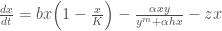

 is the prey population being harvested and
  is the predator population. Please refer to
 , rather than specific parameter values,
 ![z = [z_1, z_2, ..., z_t]](https://s0.wp.com/latex.php?latex=z+%3D+%5Bz_1%2C+z_2%2C+...%2C+z_t%5D&bg=ffffff&fg=444444&s=0&c=20201002) . The process of optimizing the parameters of a state-aware control rule is known as Direct Policy Search (DPS; Quinn et al, 2017).
. The process of optimizing the parameters of a state-aware control rule is known as Direct Policy Search (DPS; Quinn et al, 2017). , is mapped to the current prey population levels,
  by the function:
![z_{t+1} = \sum_{i=1}^n w_i \Big[exp\Big[-\Big(\frac{x_t-c_i}{b_i}\Big)^2\Big]\Big]](https://s0.wp.com/latex.php?latex=z_%7Bt%2B1%7D+%3D+%5Csum_%7Bi%3D1%7D%5En+w_i+%5CBig%5Bexp%5CBig%5B-%5CBig%28%5Cfrac%7Bx_t-c_i%7D%7Bb_i%7D%5CBig%29%5E2%5CBig%5D%5CBig%5D&bg=ffffff&fg=444444&s=0&c=20201002)
 and
and  are the center, radius, and weights of each RBF
  is the number of RBFs used in the function; in this study we use
  RBFs. With two RBFs, there are a total of 6 parameters. Increasing the number of RBFs allows for more flexible function forms to be achieved. However, two RBFs have been shown to be sufficient for this problem.
![[c_1, b_1, w_1, c_2, b_2, w_2]](https://s0.wp.com/latex.php?latex=%5Bc_1%2C+b_1%2C+w_1%2C+c_2%2C+b_2%2C+w_2%5D&bg=ffffff&fg=444444&s=0&c=20201002) ), and the current prey population, to calculate the next year’s harvesting effort.
), and the current prey population, to calculate the next year’s harvesting effort. .
.![[c_1, b_1, w_1, c_2, b_2, w_2] = [0.2, 1.1, 0.41, 0.34,0.7, 0.59]](https://s0.wp.com/latex.php?latex=%5Bc_1%2C+b_1%2C+w_1%2C+c_2%2C+b_2%2C+w_2%5D+%3D+%5B0.2%2C+1.1%2C+0.41%2C+0.34%2C0.7%2C+0.59%5D+&bg=ffffff&fg=444444&s=0&c=20201002)

![c_i, b_i, w_i \in [0,1]](https://s0.wp.com/latex.php?latex=c_i%2C+b_i%2C+w_i+%5Cin+%5B0%2C1%5D&bg=ffffff&fg=444444&s=0&c=20201002) . Below is a plot of the resulting random policy functions:
. Below is a plot of the resulting random policy functions: times, and take the average objective score over the range of simulations. This method helps to account for variability in expected outcomes due to natural stochasticity. Here, we use
  realizations of stochasticity.
 ) is calculated as:
 is the discount rate which converts future benefits to present economic value, here
  .
.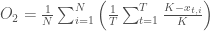


 .
.

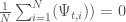


 is the time it takes the serial version of the MOEA to achieve a given hypervolume threshold, and
  is the time it takes the parallel implementation to reach the same threshold. Figure 1 below, adapted from Hadka and Reed, (2014), shows the hypervolume speedup across different parallel implementations of the Borg MOEA for the five objective NSGA II test problem run on 16,384 processors (in this work the parallel epsilon-NSGA II algorithm is used as a baseline rather than a serial implementation). Results from Figure 1 reveal that the Multi-Master implementations of Borg are able to reach each hypervolume threshold faster than the baseline algorithm and the master-worker implementation. For high hypervolume thresholds, the 16 and 32 Master implementations achieve the hypervolume thresholds 10 times faster than the baseline.


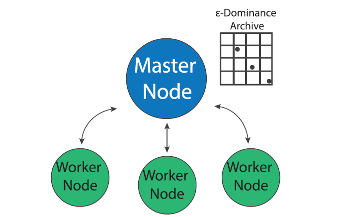


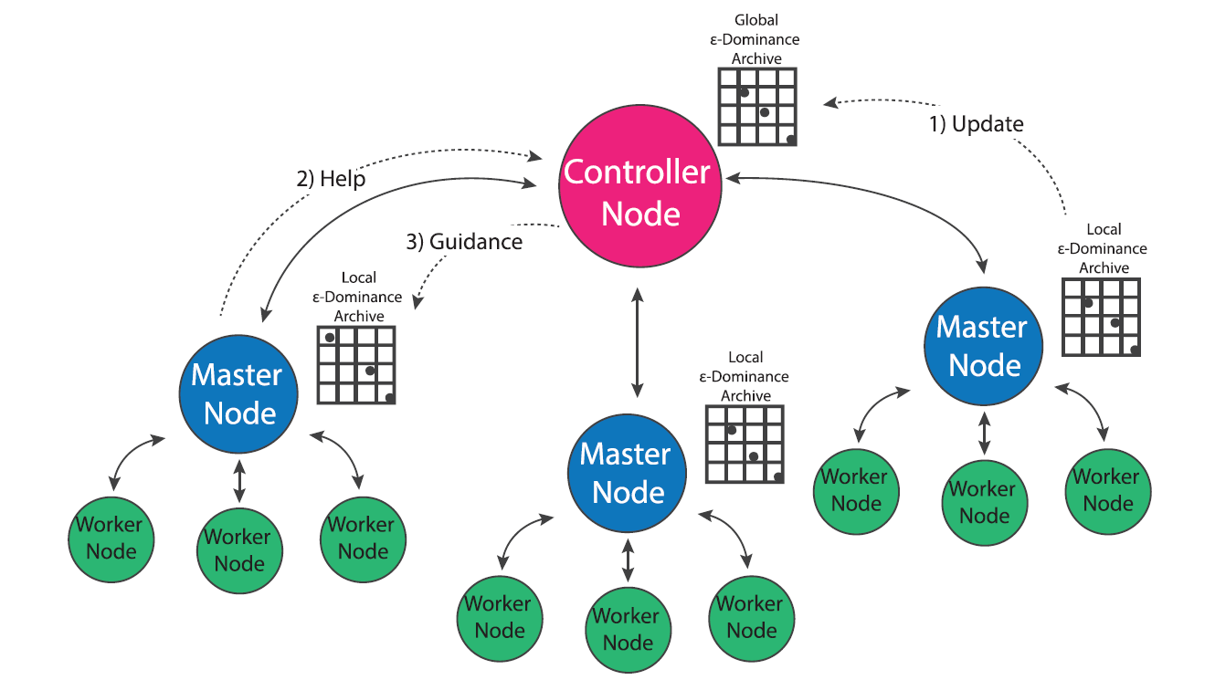


