Fisheries Training 0: Exploring Predator-Prey Dynamics

Hello there, welcome to a new training series!

In a series of five posts, we will be analyzing and exploring the Fisheries Game, which is a rich, predator-prey system with complex and nonlinear dynamics arising from the interactions between two fish species. This game will be used to walk through the steps of performing a broad a posteriori decision making process, including the exploration and characterization of impacts of system uncertain on the performance outcomes. It also serves as a conceptual tool to demonstrate the importance of accounting for deep uncertainty, and the significance of its effects on system response to management actions.

A GitHub repository containing all of the necessary code for this series is available here, and will be updated as the series develops.

We will begin here (Post 0) with an introduction to the Fisheries Game, using a modified form of the Lotka-Volterra equations for predator-prey dynamics.

Toward the end of this post, we will provide an overview of where this series is going and the tools that will be used along the way.

A very quick introduction to the Lotka-Volterra system of equations

In this game, we are stakeholders for a managed fishery. Our goal is to determine a harvesting strategy which balances tradeoffs between ecological and economic objectives. Throughout this process we will consider ecological stability, harvest yield, harvest predictability, and profits while attempting to maintain the robustness of both the ecological system and economic performance under the presence of uncertainty.

The first step in our decision making process is to model population dynamics of the fish species.

Equation 1: The base Lotka-Volterra SOE.

Equation 1 is the original Lotka-Volterra system of equations (SOE) as developed independently by Alfred Lotka in 1910, and by Vito Volterra in 1928. In this equation, x is the population density of the prey, and y is the population density of the predator. This SOE characterizes a prey-dependent predator-prey functional response, which assumes a linear relationship between prey consumption and predator growth.

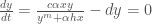
Arditi and Akçakaya (1990) constructed an alternative predator-prey SOE, which assume a non-linear functional response (i.e., predator population growth is not linear with consumption). It accounts for predation efficiency parameters such as interference between predators, time needed to consume prey after capture, and a measure of how long it takes to convert consumed prey into new predators. This more complex SOE takes the form:

Equation 2: The full predator-dependent predator-prey SOE, including predator interference (m) and harvesting (z).

The full description of the variables are as follows: x and y are the prey and predator population densities at time t respectively (where t is in years); α is the rate at which the predator encounters the prey; b is the prey growth rate; c is the rate at which the predator converts prey to new predators; d is predator death rate; h is the time it needs to consume the prey (handling time); K is the environmental carrying capacity; m is the level of predator interaction; and z is the fraction of the prey population that is harvested. In this post, we will spend some time exploring the potential behavior of these equations.

Before proceeding further, here are some key terms used throughout this post:

• Zero isoclines: Lines on the plot indicating prey or predator population levels that result in constant population size over time (zero growth rate).
• Global attractor: The specific value that the system tends to evolve toward, independent of initial conditions.
• Equilibrium point: The intersection of two (or more) zero isoclines; a point or line of trajectory convergence.
  • Stable (nontrivial) equilibrium: Equilibrium at which both prey and predator exist
  • Unstable equilibrium: Global attractor is a stable limit cycle
• Stable limit cycle: A closed (circular) trajectory
• Trajectory: The path taken by the system given a specific set of initial conditions.
• Functional response: The rate of prey consumption by your average predator.

Population equilibrium and stability

When beginning to consider a harvesting policy, it is important to first understand the natural stability of the system.

Population equilibrium is a necessary condition for stability. The predator and prey populations are in equilibrium if the rate of change of the populations is zero:

Predator stability

Let’s first consider the equilibria of the predator population. In this case, we are only interested in the non-trivial (or co-existence) equilibria where the predator and prey populations are non-zero (, and ).

Here, we are interested in solving for the predator zero-isocline () which satisfies this equation. Re-arrangement of the above equation yields:

Solving for yields the predator zero-isocline:

In the context of the fisheries, we are interested in the co-existence conditions in which . From the zero-isocline stability equation above, it is clear that this is only true if:

Simply put, the rate at which predators convert prey into new predators () must be greater than the death rate () scaled by the time it needs to consume prey ().

Prey stability

A similar process can be followed for the derivation of the zero-isocline stability condition for the prey population. The stability condition can be determined by solving for:

As the derivation of the prey isocline is slightly more convoluted than the predator isocline, the details are not presented here, but are available in the Supplementary Materials of Hadjimichael et al. (2020), which is included in the GitHub repository for this post here.

Resolution of this stability condition yields the second necessary co-existence equilibrium condition:

Uncertainty

As indicated by the two conditions above, the stability of the predator and prey populations depends upon ecosystem properties (e.g., the availability of prey, , predator interference, , and the carrying capacity, ), unique species characteristics (e.g., the prey growth rate, , and predation efficiency parameters , ).

Specification of different values for these parameters results in wildly different system dynamics. Below are examples of three different population trajectories, each generated using the same predator-dependent system of equations, with different parameter values.

Figure 1: Three trajectory fields, resulting from predator-prey models with different parameter values. (a) A stable equilibrium with a single global attractor (values: a = 0.01, b = 0.35, c = 0.60, d = 0.20, h = 0.44, K = 1900, m = 0.30, z = 0.0); (b) an unstable system with limit cycles as global attractors (values: a = 0.32, b = 0.48, c = 0.40, d = 0.16, h = 0.23, K = 2400, m = 0.30, z = 0.0); (c) an unstable system with deterministic extinction of both species (values: a = 0.61, b = 0.11, c = 0.80, = 0.18, h = 0.18, K = 3100, m = 0.70, z = 0.0).

Exploring system dynamics (interactive!)

To emphasize the significance of parameter uncertainty on the behavior of predator-prey system behavior, we have prepared an interactive Jupyter Notebook. Here, you have ability to interactively change system parameter values and observe the subsequent change in system behavior.

The Binder link to the interactive Jupyter Notebook prepared by Trevor Amestoy can be found here. Before the code can be run, open the ‘Terminal’, as shown in Figure 2 below.

Figure 2: Starting page of the Jupyter Notebook binder.

Install the necessary libraries by entering the following line into the terminal:

pip install numpy scipy matplotlib pandas

You’re good to go once the libraries have been loaded. Open the Part_0_Interactive_fisheries_ODEs.ipynb file in the Part_0_ODE_Dynamics/ folder.

Play around with the sliders to see what system trajectories you end up with! Notice how abruptly the population dynamics change, even with minor changes in parameter values.

The following GIFs show some potential trajectories you might observe as you vary the ranges of the variables:

Starting at a stable equilibrium

In Figure 3 below, both prey and predator eventually coexist at constant population sizes with no human harvesting.

Figure 3: The Fisheries system at a stable equilibrium quickly transitioning to an unstable equilibrium, and back again to a stable equilibrium.

However, this is a fishery with very small initial initial prey population size. Here, note how quickly the system changes from one of stable equilibrium into that of unstable equilibrium with a small decrease in the value of α. Without this information, stakeholders might unintentionally over-harvest the system, causing the extinction of the prey population.

Starting at an unstable equilibrium

Next, Figure 4 below shows an unstable equilibrium with limit cycles and no human harvesting.

Figure 4: An unstable equilibrium where the both prey and predator populations oscillate in a stable limit cycle.

Figure 4 shows that a system will be in a state of unstable equilibrium when it takes very little time for the predator to consume prey, given moderately low prey population sizes and prey population growth rate. Although predators die at a relatively high rate, the prey population still experiences extinction as it is unable to replace population members lost through consumption by the predator species. This is a system in which stakeholders might instead choose to harvest the predator species.

Introducing human harvesting

Finally, a stable equilibrium that changes when human harvesting of the prey population is introduced in Figure 5 below.

Figure 5: An unstable equilibrium where the both prey and predator populations oscillate in a stable limit cycle.

This Figure demonstrates a combination of system parameters that might represent a system that can be harvested in moderation. It’s low prey availability is abated by a relatively high predator growth rate and relatively low conversion rates. Be that as it may, exceeding harvesting rates may suddenly cause the system to transition into an unstable equilibrium, or in the worst case lead to an unexpected collapse of the population toward extinction.

Given that the ecosystem parameters are uncertain, and that small changes in the assumed parameter values can result in wildly different population dynamics, it begs the question: how can fisheries managers decide how much to harvest from the system, while maintaining sustainable population levels and avoiding system collapse?

This is the motivating question for the upcoming series!

The MSD UC eBook

To discover economic and environmental tradeoffs within the system, reveal the variables shaping the trajectories shown in Figure 3 to 5, and map regions of system vulnerability, we will need suitable tools.

In this training series, we will be primarily be using the MSD UC eBook and its companion GitHub repository as the main resources for such tools. Titled ‘Addressing uncertainty in MultiSector Dynamics Research‘, the eBook is part of an effort towards providing an open, ‘living’ toolkit of uncertainty characterization methods developed by and for the MultiSector Dynamics (MSD) community. The eBook also provides a hands-on Jupyter Notebook-based tutorial for performing a preliminary exploration of the dynamics within the Fisheries Game, which we will be expanding on in this tutorial series. We will primarily be using the eBook to introduce you to sensitivity analysis (SA) methods such as Sobol SA, sampling techniques such as Latin Hypercube Sampling, scenario discovery approaches like Logistic Regression, and their applications to complex, nonlinear problems within unpredictable system trajectories. We will also be making frequent use of the functions and software packages available on the MSD GitHub repository.

To make the most out of this training series, we highly recommend familiarizing yourself with the eBook prior to proceeding. In each of the following posts, we will also be making frequent references to sections of the eBook that are relevant to the current post.

Training sequence

In this post, we have provided an overview of the Fisheries Game. First, we introduced the basic Lotka-Volterra equations and its predator-dependent predator-prey variation (Arditi and Akcakaya, 1990) used in Hadjimichael et al. (2020). We also visualized the system and explored how the system trajectories change with different parameter specifications. Next, we introduced the MSD UC eBook as a toolkit for exploring the Fisheries’ system dynamics.

Overall, this post is meant to be a gateway into a deep dive into the system dynamics of the Fisheries Game as formulated in Hadjimichael et al. (2020), using methods from the UC eBook as exploratory tools. The next few posts will set up the Fisheries Game and its objectives for optimization, explore the implications of varying significant decision variables, map parameter ranges that result in system vulnerability, and visualize these outcomes. The order for these posts are as follows:

Post 1 Problem formulation and optimization of the Fisheries Game in Rhodium

Post 2 Visualizing and exploring the Fisheries’ Pareto set and Pareto front using Rhodium and J3

Post 3 Identifying important system variables using different sensitivity analysis methods

Post 4 Mapping consequential scenarios that drive the Fisheries’ vulnerability to deep uncertainty

That’s all from us – see you in Post 1!

References

Abrams, P., & Ginzburg, L. (2000). The nature of predation: prey dependent, ratio dependent or neither?. Trends In Ecology &Amp; Evolution, 15(8), 337-341. https://doi.org/10.1016/s0169-5347(00)01908-x

Arditi, R., & Akçakaya, H. R. (1990). Underestimation of Mutual Interference of Predators. Oecologia, 83(3), 358–361. http://www.jstor.org/stable/4219345

Hadjimichael, A., Reed, P., & Quinn, J. (2020). Navigating Deeply Uncertain Tradeoffs in Harvested Predator-Prey Systems. Complexity, 2020, 1-18. https://doi.org/10.1155/2020/4170453

Lotka, A. (1910). Contribution to the Theory of Periodic Reactions. The Journal Of Physical Chemistry, 14(3), 271-274. https://doi.org/10.1021/j150111a004

Reed, P.M., Hadjimichael, A., Malek, K., Karimi, T., Vernon, C.R., Srikrishnan, V., Gupta, R.S., Gold, D.F., Lee, B., Keller, K., Thurber, T.B, & Rice, J.S. (2022). Addressing Uncertainty in Multisector Dynamics Research [Book]. Zenodo. https://doi.org/10.5281/zenodo.6110623

Volterra, V. (1928). Variations and Fluctuations of the Number of Individuals in Animal Species living together. ICES Journal Of Marine Science, 3(1), 3-51. https://doi.org/10.1093/icesjms/3.1.3

MORDM VII: Optimality, robustness, and reevaluation under deep uncertainty

In the previous MORDM post, we visualized the reference set of performance objectives for the North Carolina Research Triangle and conducted a preliminary multi-criterion robustness analysis using two criteria: (1) regional reliability should be at least 98%, and (2) regional restriction frequency should be not more than 20%. Using these metrics, we found that Pareto-optimality does not guarantee satisfactory robustness, a statement that is justified by showing that not all portfolios within the reference set satisfied the robustness criteria.

In this post, we will explain the differences between optimality and robustness, and justify the importance of robust optimization instead of sole reliance on a set of optimal solutions (aka an optimal portfolio). To demonstrate the differences better, we will also reevaluate the Pareto optimal set of solutions under a more challenging set of states of the world (SOWs), a method first used in Herman et al (2013, 2014) and Zeff et al (2014). The formal term for this method, Deeply Uncertain (DU) Re-evaluation was coined in a 2019 paper by Trindade et al.

Optimality vs robustness

The descriptions of optimality are many. From a purely technical perspective, a Pareto optimal set is a set of decision variables or solutions that maps to a Pareto front, or a set of performance objectives where improving one objective cannot be improved without causing performance degradation in another. For the purposes of this blog post, we shall use the definition of optimality as laid out by Beyer and Sendoff in their 2007 paper:

The global optimal design…depends on the…(objective) functions and constraints…however, these functions always represent models and/or approximations of the real world.

Beyer and Sendhoff (2007)

In other words, a Pareto reference set is only optimal within the bounds of the model it was generated from. This makes sense; models are only approximations of the real world. It is difficult and computationally expensive to have bounds on the degree of certainty to which the model optimum maps to the true optimum due to uncertainties driven by human action, natural variability, and incomplete knowledge. Optimization is static in relation to reality – the set of solutions found do not change with time, and only account for the conditions within the model itself. Any deviation from this set of solutions or unaccounted differences between the actual system and model may result in failure (Herman et al, 2015; Read et al 2014).

This is why searching the set of optimal solutions for robust solutions is important. Herman et al (2015) quotes an earlier works by Matalas and Fiering (1977) that defines robustness as the insensitivity a system’s portfolio to uncertainty. Within the MORDM context, robustness was found to be best defined using the multi-criterion satisficing robustness measure (Herman et al, 2015), which refers to the ability of a solution to meet one or more requirements (or criteria) set by the decision-makers when evaluated under a set of challenging scenarios. More information on alternative robustness measures can be found here.

In this blog post, we will begin to explore this concept of robustness by conducting DU Re-evaluation, where we will perform the following steps:

Generate a set of ROF tables from a more challenging set of SOWs

Recall that we previously stored our Pareto-optimal solution set in a .csv file names ‘NC_refset.csv’ (find the original Git Repository here). Now, we will write a quick Python script (called rof_tables_reeval.py in the Git Repository) using MPI4PY that will parallelize and speed up the ROF table generation and the bash script to submit the job. More information on parallelization using MPI4PY can be found in this handy blog post by Dave Gold.

First, create a Python virtual environment within the folder where all your sourcecode is kept and activate the virtual environment. I called mine python3_venv:

python3 -m venv python_venv
source python_venv/bin/activate

Next, install the numpy and mpi4py libraries:

pip install numpy mpi4py

Then write the Python script as follows:

# -*- coding: utf-8 -*-
"""
Created on Tues March 1 2022 16:16
@author: Lillian Bei Jia Lau
"""

from mpi4py import MPI
import numpy as np
import subprocess, sys, time
import os

# 5 nodes, 50 RDMs per node
# 16 tasks per node
# 5 RDMs per task
comm = MPI.COMM_WORLD
rank = comm.Get_rank() # up to 20 processes
print('rank = ', rank)

N_RDMs_needed = 100
N_REALIZATIONS = 100
N_RDM_PER_NODE = 20
N_TASKS_PER_NODE = 10 
N_RDM_PER_TASK = 2 # each task handles two RDMs
N_TASKS = 50 # rank ranges from 0 to 50

DATA_DIR = "/scratch/lbl59/blog/WaterPaths/"
SOLS_FILE_NAME = "NC_dvs_all_noheader.csv"
N_SOLS = 1

OMP_NUM_THREADS = 32

for i in range(N_RDM_PER_TASK):
    current_RDM = rank + (N_TASKS * i)

    command_gen_tables = "./waterpaths -T {} -t 2344 -r {} -d {} -C 1 -O rof_tables_reeval/rdm_{} -e 0 \
            -U TestFiles/rdm_utilities_test_problem_reeval.csv \
            -W TestFiles/rdm_water_sources_test_problem_reeval.csv \
            -P TestFiles/rdm_dmp_test_problem_reeval.csv \
            -s {} -f 0 -l {} -R {}\
            -p false".format(OMP_NUM_THREADS, N_REALIZATIONS, DATA_DIR, current_RDM, SOLS_FILE_NAME, N_SOLS, current_RDM)

    print(command_gen_tables)
    os.system(command_gen_tables)

comm.Barrier()

Before proceeding, a quick explanation on what all this means:

• Line 12: We are parallelizing this job across 5 nodes on Cornell’s THECUBE (The Cube) computing cluster.
• Lines 19-28: On each node, we are submitting 10 tasks to each of the 5 nodes requested. Each task, in turn, is handling 2 robust decision-making (RDM) multiplier files that scale up or scale down a hydroclimatic realization make a state of the world more (or less) challenging. In this submission, we are creating 400 different variations of each hydroclimatic scenario using the 400 RDM files, and running it across only one solution
• Line 16 and 31: The ‘rank’ is the order of the tasks in which there are submitted. Since there are 10 tasks over 5 nodes, there will be a total of 50 tasks being submitted. Note and understand how the current_RDM is calculated.
• Lines 32 to 37: This is the command that you are going to submit to The Cube. Note the -C and -O flags; a value of 1 for the -C flag tells WaterPaths to generate ROF tables, and the -O tells WaterPaths to output each ROF table file into a folder within rof_tables_reeval/rdm_{}for each RDM. Feel free to change the filenames as you see fit.

To accompany this script, first create the following folders: output, out_reeval, and rof_tables_reeval. The output folder will contain the simulation results from running the 1 solution across the 100 hydroclimatic realizations. The out_reeval folder will store any output or error messages such as script runtime.

Then, write the following bash submission script:

#!/bin/bash
#SBATCH -n 50 -N 5 -p normal
#SBATCH --job-name=rof_tables_reeval
#SBATCH --output=out_reeval/rof_tables_reeval.out
#SBATCH --error=out_reeval/rof_tables_reeval.err
#SBATCH --time=200:00:00
#SBATCH --mail-user=lbl59@cornell.edu
#SBATCH --mail-type=all

export OMP_NUM_THREADS=32

module load openmpi3/3.1.4
module spider py3-mpi4py
module spider py3-numpy/1.15.3

START="$(date +%s)"

mpirun python3 rof_tables_reeval.py

DURATION=$[ $(date +%s) - ${START} ]

echo ${DURATION}

You can find the bash script under the filename rof_table_gen_reeval.sh. Finally, submit the script using the following line:

sbatch ./rof_table_gen_reeval.sh

The run should take roughly 5 hours. We’re good for some time!

Re-evaluate your solutions (and possibly your life choices, while you’re at it)

Once the ROF tables are generated, it’s time to get a little hands-on with the underlying WaterPaths code. Navigate to the following PaperTestProblem.cpp file using:
cd /yourfilepath/WaterPaths/src/Problem/

Follow the next steps carefully.

1. Delete PaperTestProblem.cpp and replace it with the file PaperTestProblem-reeval.cpp. It can be found in the the main Git Repository.
2. Rename the latter file PaperTestProblem.cpp – it will be the new PaperTestProblem file that will be able to individually read each RDM scenario’s ROF tables.
3. Re-make WaterPaths by calling make clean and then make gcc in the command line. This will ensure that WaterPaths has no problems running the new PaperTestProblem.cpp file.

Next, write the following Python script (called run_du_reeval.py in the Git repository):

# -*- coding: utf-8 -*-
"""
Created on Tues March 1 2022 16:16

@author: Lillian Bei Jia Lau
"""

from mpi4py import MPI
import numpy as np
import subprocess, sys, time
import os

N_RDMs_needed = 100  # N_TASKS_PER_NODE * N_RDM_PER_TASK * num nodes
N_REALIZATIONS = 100
N_RDM_PER_NODE = 20
N_TASKS_PER_NODE = 10 # rank ranges from 0 to 15
N_RDM_PER_TASK = 2 # each task handles five RDMs
N_TASKS = 50

comm = MPI.COMM_WORLD
rank = comm.Get_rank() # up to 20 processes
print('rank = ', rank)

DATA_DIR = "/scratch/lbl59/blog/WaterPaths/"
SOLS_FILE_NAME = "NC_dvs_all_noheader.csv"
N_SOLS = 69
OMP_NUM_THREADS = 32

for i in range(N_RDM_PER_TASK):
    current_RDM = rank + (N_TASKS * i)

    command_run_rdm = "./waterpaths -T {} -t 2344 -r {} -d {} -C -1 -O rof_tables_reeval/rdm_{} -e 0 \
            -U TestFiles/rdm_utilities_test_problem_reeval.csv \
            -W TestFiles/rdm_water_sources_test_problem_reeval.csv \
            -P TestFiles/rdm_dmp_test_problem_reeval.csv \
            -s {} -R {} -f 0 -l 69\
            -p false".format(OMP_NUM_THREADS, N_REALIZATIONS, DATA_DIR, \
                    current_RDM , SOLS_FILE_NAME, current_RDM)

    print(command_run_rdm)
    os.system(command_run_rdm)

comm.Barrier()

Note the change in the -C flag; its value is now -1, telling WaterPaths that it should import the ROF table values from the folder indicated by the -O flag. The resulting objective values for each RDM will be saved in the output folder we previously made.

The accompanying bash script, named du_reeval.sh is as follows:

#!/bin/bash
#SBATCH -n 50 -N 5 -p normal
#SBATCH --job-name=mordm_training_du_reeval
#SBATCH --output=out_reeval/mordm_training_du_reeval.out
#SBATCH --error=out_reeval/mordm_training_du_reeval.err
#SBATCH --time=200:00:00
#SBATCH --mail-user=lbl59@cornell.edu
#SBATCH --mail-type=all

export OMP_NUM_THREADS=32
module load openmpi3/3.1.4
module spider py3-numpy/1.15.3

START="$(date +%s)"

mpirun python3 run_du_reeval.py

DURATION=$[ $(date +%s) - ${START} ]

echo ${DURATION}

This run should take approximately three to four days. After that, you will have 1000 files containing 69 objective value sets resulting from running the 69 solutions across 1000 deeply-uncertain states of the world.

Summary

In this post, we defined optimality and robustness. We demonstrated how to run a DU re-evaluation across 100 challenging SOWs to observe how these ‘optimal’ solutions perform in more extreme scenarios. This is done to show that optimality is bound by current model states, and any deviation from the expected circumstances as defined by the model may lead to degradations in performance.

In the next blog post, we will be visualizing these changes in performance using a combination of sensitivity analysis, scenario discovery, and tradeoff analysis.

References

Beyer, H. and Sendhoff, B., 2007. Robust optimization – A comprehensive survey. Computer Methods in Applied Mechanics and Engineering, 196(33-34), pp.3190-3218.

Herman, J., Reed, P., Zeff, H. and Characklis, G., 2015. How Should Robustness Be Defined for Water Systems Planning under Change?. Journal of Water Resources Planning and Management, 141(10), p.04015012.

Herman, J., Zeff, H., Reed, P. and Characklis, G., 2014. Beyond optimality: Multistakeholder robustness tradeoffs for regional water portfolio planning under deep uncertainty. Water Resources Research, 50(10), pp.7692-7713.

Matalas, N. C., and Fiering, M. B. (1977). “Water-resource systems planning.” Climate, climatic change, and water supply, studies in geophysics, National Academy of Sciences, Washington, DC, 99–110.

Read, L., Madani, K. and Inanloo, B., 2014. Optimality versus stability in water resource allocation. Journal of Environmental Management, 133, pp.343-354.

Zeff, H., Kasprzyk, J., Herman, J., Reed, P. and Characklis, G., 2014. Navigating financial and supply reliability tradeoffs in regional drought management portfolios. Water Resources Research, 50(6), pp.4906-4923.

Factor prioritization and factor fixing: how to know what’s important

There have been several blogposts on sensitivity analysis (SA) on this blog, focusing primarily on tools to perform it (e.g., SALib) and visualize outputs. Today I’ll be providing some more information on how to decide which factors are most important in affecting our output and which are largely inconsequential. Picking what is actually important for what we care about is obviously largely subjective and case-dependent, but this post is meant to provide some support to that exercise. I will performing a Global Sensitivity Analysis of a system resulting in a rank-ordering of the most important factors driving variability in the output (i.e., factor prioritization), which can be used to decide which are the least influential factors that can be fixed to simplify the model (i.e., factor fixing) [1].

The scripts I’ll be using can be found here, and I’ll be using a fishery model to demonstrate, as a simplified representation of a socio-ecological system we’re trying to manage. The procedure I’ll be following has been based on the work found in [2-4].

The idea is this:
I generate 1000 samples of uncertain factors that might be driving variability in my outcome (let’s call this Set 1). I apply a certain SA method on the samples and the outcomes and get sensitivity indices for each of my factors, ranking them from most important to least. Where do I draw the line between important and not important?
We can create a Set 2, using only the T most important factors from our Set 1 sample, and fixing all other factors to their default values.
We can also create a Set 3, now fixing the T most important factors to defaults and using the sampled values of all other factors from Set 1.

If we classified our important and unimportant factors correctly, then the correlation coefficient between the model outputs of Set 2 and Set 1 should approximate 1 (since we’re fixing all factors that don’t matter), and the correlation coefficient between outputs from Set 3 and Set 1 should approximate 0 (since the factors we sampled are inconsequential to the output).

Here’s how it’s done using SALib and the Delta Method (in the interest of space I’ll only share the most important snippets of code, you need the full scripts to make it run, which are in this repository) :

First we set up our problem using SALib nomenclature, generate 1000 samples using all factors (which will be our Set 1) and run the model for all 1000 samples. Finally we analyze our output using the Delta method. (This should take a couple minutes to run on your personal computer.)

# Set up dictionary with system parameters
problem = {
  'num_vars': 9,
  'names': ['a', 'b', 'c', 'd','h',
            'K','m','sigmaX','sigmaY'],
  'bounds': [[ 0.002, 2],
             [0.005, 1],
             [0.2, 1],
             [0.05, 0.2],
             [0.001, 1],
             [100, 5000],
             [0.1, 1.5],
             [0.001, 0.01],
             [0.001, 0.01]]
}

defaultvalues = np.array([0.005, 0.5, 0.5, 0.1, 0.1, 2000, 0.7, 0.004, 0.004])

# Generate samples
nsamples = 1000
X_Set1 = latin.sample(problem, nsamples) # This is Set 1

# Run model for all samples
output = [fish_game(*X_Set1[j,:]) for j in range(nsamples)]

# Perform analysis
results = delta.analyze(problem, X_Set1, np.asarray(output), print_to_console=True)

This will produce output like below, telling as the Delta indices of each of the sampled parameters, the confidence internals of those, the First order Sobol indices of the parameters, and their equivalent confidence intervals.

Parameter delta delta_conf S1 S1_conf
a 0.102206 0.021648 0.052453 0.033510
b 0.139056 0.018379 0.065019 0.022922
c 0.090550 0.016505 0.006749 0.007823
d 0.076542 0.005375 0.003923 0.009140
h 0.097057 0.016910 0.021070 0.009275
K 0.267461 0.020434 0.190670 0.057397
m 0.252351 0.040149 0.315562 0.031664
sigmaX 0.076175 0.014001 0.005930 0.005333
sigmaY 0.075390 0.015346 0.004970 0.011557

Without further analysis, one simple way of determining whether a parameter is unimportant is to check whether the confidence interval of its value overlaps 0 (i.e., subtract delta_conf from delta). For our particular results, this doesn’t seem to be the case for any of our delta values, though it does happen for some of the S1 values (c, d, sigmaY). You can refer to this post for discussion on what this might mean.
Looking at the delta values, we can clearly see two factors coming up top (K and m), followed by b, and a closely behind it. The rest of the parameters are reduced in their importance in small decrements after that. So where should we draw the line of importance? Another simple way is to use a threshold (say, 0.1) as a cutoff value [3], but one could argue over including a and not h, given how close their indices are and the wider confidence interval of a (see also the appendix below on this).

But, let’s continue with our analysis. What I am doing below is the following. First, I sort the factors from most to least important based on my results for the delta indices. Then, I create my Sets 2 and 3 on which I’ll be iteratively replacing the values of important factors with either those from Set 1 or with defaults. Finally, I loop through all possible numbers of important factors (1 to 9), generate Sets 2 and 3, calculate outputs for all samples in each, and calculate their correlation with the outputs from Set 1. (This should take 20-30 minutes to run on your personal computer.)

# Sort factors by importance
factors_sorted = np.argsort(results['delta'])[::-1]

# Set up DataFrame of default values to use for experiment
X_defaults = np.tile(defaultvalues,(nsamples, 1))

# Create initial Sets 2 and 3
X_Set2 = np.copy(X_defaults)
X_Set3 = np.copy(X_Set1)

for f in range(1, len(factors_sorted)+1):
    ntopfactors = f
    
    for i in range(ntopfactors): #Loop through all important factors
        X_Set2[:,factors_sorted[i]] = X_Set1[:,factors_sorted[i]] #Fix use samples for important
        X_Set3[:,factors_sorted[i]] = X_defaults[:,factors_sorted[i]] #Fix important to defaults
    
    # Run model for all samples    
    output_Set2 = [fish_game(*X_Set2[j,:]) for j in range(nsamples)]
    output_Set3 = [fish_game(*X_Set3[j,:]) for j in range(nsamples)]
    
    # Calculate coefficients of correlation
    coefficient_S1_S2 = np.corrcoef(output,output_Set2)[0][1]
    coefficient_S1_S3 = np.corrcoef(output,output_Set3)[0][1]

I can also plot the outputs from each iteration, which should look something like this (this is animated to show all figures, in the interest of space):

The figures above tell us the following:
If we choose one important factor (K) and fix all other parameters our outputs don’t really capture the variability of outcomes produced when considering all nine (this is also a case against one-at-a-time type analyses). The coefficient of correlation between Sets 1 and 2 is pretty low (0.44) suggesting we’re still missing important parameters. We’re doing a better job by actually fixing our most important parameter and varying all others (figure on the right, with R=0.763).
Adding the second most important factor (m), shifts things significantly to the right direction, by increasing our coefficient on the right and reducing the one on the left to R=0.203.
There is only a slight improvement with the addition of the third factor (b), but with the inclusion of the fourth (a), our reduced model is already looking very close to the full, with R=0.94. Our counter model excluding these four factors (on the right) also has a very low coefficient of R=0.025.
One could consider this performance sufficient, with the model reduced to four parameters instead of nine. Further adding parameter h and then c would further improve the values to a near perfect match between Set 2 and Set 1, but this is where subjectivity takes over, depending on the cost of adding these variables and how much we care about fidelity in this case.
It is also clear that it is likely safe to fix the last three parameters, as in this case they don’t have any consequential effects on our outcomes.

References:
[1] Saltelli, Andrea, et al.  Global Sensitivity Analysis: The Primer. (2008)
[2] T. H. Andres, “Sampling methods and sensitivity analysis for large parameter sets,” Journal of Statistical Computation and Simulation, vol. 57, no. 1–4, pp. 77–110, Apr. 1997, doi: 10.1080/00949659708811804.
[3] Y. Tang, P. Reed, T. Wagener, and K. van Werkhoven, “Comparing sensitivity analysis methods to advance lumped watershed model identification and evaluation,” Hydrology and Earth System Sciences, vol. 11, no. 2, pp. 793–817, Feb. 2007, doi: https://doi.org/10.5194/hess-11-793-2007.
[4] J. Nossent, P. Elsen, and W. Bauwens, “Sobol’ sensitivity analysis of a complex environmental model,” Environmental Modelling & Software, vol. 26, no. 12, pp. 1515–1525, Dec. 2011, doi: 10.1016/j.envsoft.2011.08.010.

---

Appendix:
Another way to identify a threshold of importance to classify parameters, is to add a dummy parameter to your model, that does nothing. Reperforming my SA for this same system including the dummy, produces this:

Parameter delta delta_conf S1 S1_conf
a 0.105354 0.019236 0.040665 0.020949
b 0.144955 0.023576 0.050471 0.014810
c 0.075516 0.009578 0.003889 0.006113
d 0.081177 0.011604 0.004186 0.007235
h 0.101583 0.010008 0.032759 0.021343
K 0.261329 0.022876 0.174340 0.038246
m 0.258345 0.024750 0.325690 0.052234
sigmaX 0.071862 0.008620 0.001681 0.006720
sigmaY 0.077337 0.009344 0.003131 0.006918
dummy 0.072546 0.008313 0.004176 0.009567

Even though the dummy does absolutely nothing in our model, it was still given a non-zero delta index by the analysis (0.07). One could use this as the cutoff value of non-importance and choose to fix parameters c, sigmaX, and sigmaY.

Spatial and temporal visualization of water demands in a basin

One of my main projects in the last couple years has been in the Upper Colorado River Basin, where we’ve been investigating how hundreds of water users in the basin might be affected by a variety of different changes and uncertainties that might take place in the region. Being in Colorado, water allocation in the basin follows prior-appropriation, where every user has a certain water right, defined by its seniority (where more senior = better) and its decree (i.e. how much water the right is granted for extraction). For the different users in the basin to receive water for their respective uses, prior-appropriation determines who gets X amount of water first based on seniority and given water availability, and then repeats down the seniority order until all requested water has been allocated. Hence, no user can extract water in a manner that affects any senior to them user.

During this investigation, we’ve been interested in seeing how this actually plays out through time and space in the basin, with the aim of potentially better understanding any consequential relationships that might exist between different users, as well as any emerging patterns that might be missed by looking at the data in a different manner. I tried to write a little script to do this in Python. I will be visualizing how users along the basin requested for some water at some historical month (the demand) and how much of that demand was actually met (the shortage), based on their right seniority and water availability in the basin.

There have been multiple posts in the blog on generating maps in Python (as well as in other languages), and they all use a module called Basemap which has been the most popular for these things, but it’s kinda buggy, and kinda a pain to install, and kinda a pain to get working, and I spent the better part of an entire workday to re-set it up on my machine and couldn’t. Enter Cartopy. After Basemap was announced deprecated, Cartopy was meant to be its replacement so I decided to transition. It was super easy to install and start generating maps within a couple minutes and the code I’ll be sharing today will be using that. I will also be using matplotlib’s animation classes to capture the water allocation to the different users through time in a video or a GIF.

First, I load up all necessary packages and data. structures contains the X and Y coordinates of all the diversion points; demands and shortages contain monthly data of water demand and shortage for each diversion point.

import numpy as np
import cartopy.feature as cpf
import cartopy.crs as ccrs
import matplotlib.pyplot as plt
import cartopy.io.img_tiles as cimgt
import pandas as pd
import matplotlib.animation as animation
import math

structures = pd.read_csv('modeled_diversions.csv',index_col=0)
demands = pd.read_csv('demands.csv',index_col=0)
shortages = pd.read_csv('shortages.csv',index_col=0)

Then, I set up the extent of my map (i.e., the region I would like to show). rivers_10m loads the river “feature” at a 10m resolution. There’s a lot of different features that can be added (coastlines, borders, etc.). Finally, I load the tiles which is basically the background map image (many other options also).

extent = [-109.069,-105.6,38.85,40.50]
rivers_10m = cpf.NaturalEarthFeature('physical', 'rivers_lake_centerlines', '10m')
tiles = cimgt.StamenTerrain()

I draw the figure more or less as I would in matplotlib, using the matplotlib scatter to draw my demand and shortage points. The rest of the lines are basically legend customization by creating dummy artists to show max demands and shortages in the legend.

fig = plt.figure(figsize=(12, 6))
ax = plt.axes(projection=tiles.crs)
ax.add_feature(rivers_10m, facecolor='None', edgecolor='b')
ax.add_image(tiles, 9, interpolation='none')
ax.set_extent(extent)
dem_points = ax.scatter(structures['X'], structures['Y'], marker = '.', s = demands['0']/50, c = 'dodgerblue', transform=ccrs.Geodetic())
short_points = ax.scatter(structures['X'], structures['Y'], marker = '.', s = shortages['0']/50, c = 'coral' ,transform=ccrs.Geodetic())
l2 = ax.scatter(-110,37, s=demands.values.max()/50, c = 'dodgerblue', transform=ccrs.Geodetic())
l4 = ax.scatter(-110,37, s=shortages.values.max()/50, c = 'coral',transform=ccrs.Geodetic())
dem_label = ax.scatter(-110,37, s=0, transform=ccrs.Geodetic())
short_label = ax.scatter(-110,37, s=0, transform=ccrs.Geodetic())
labels = ['Max Demand' , str(demands.values.max()) + ' af', 
          'Max Shortage' , str(shortages.values.max()) + ' af']
legend = ax.legend([dem_label, l2, short_label, l4], labels, ncol=2, loc = 'upper left', title = 'Month: '+ str((0 + 10) % 12 +1) + '/' + str(int(math.floor(0/12))+1908)+'\n', fontsize=10, title_fontsize = 14, borderpad=2, handletextpad = 1.3)

This code should produce something like the following, which shows the relative demand across users in blue, as well as how much of that demand was not met (shortage) in orange for November 1908. The large circles in the legend show the max demand and shortage across all users across all months in the record for reference.

To animate this, it’s very simple. All we need to create is another function (in this case update_points) that will define what changes at every frame of the animation. I’ve defined my function to adjust the size of every circle according to the timestep/frame, as well as change the title of the legend to the correct month. Matplotlib’s FuncAnimation then uses that and my figure to update it repeatedly (in this case for 120 steps). Finally, the animation can be saved to a video.

def update_points(num, dem_points, short_points, legend):
    dem_points.set_sizes(demands[str(num)]/10)
    short_points.set_sizes(shortages[str(num)]/10)
    legend.set_title('Month: '+ str((num + 10) % 12 +1) + '/' + str(int(math.floor(num/12))+1908))
    return dem_points, short_points, legend 
       
anim = animation.FuncAnimation(fig, update_points, 120, fargs=(dem_points, short_points, legend),
                                   interval=200, blit=False)
anim.save('basin_animation.mp4', fps=10,  dpi=150, extra_args=['-vcodec', 'libx264'])

WordPress reduces resolution, full res can be found here: https://imgur.com/a/6zfYIDU

There’s a lot to be added and improved, but from this simple version we can immediately see certain diversions popping out as well as geographical regions that exhibit frequent shortage. I will continue working on this and hopefully share improved versions in the future.