Parallel Programming Part 2: Demonstrating OpenMP constructs with a simple test case

Parallel Programming Part 2: Demonstrating OpenMP constructs with a simple test case

In Parallel Programming Part 1, I introduced a number of basic OpenMP directives and constructs, as well as provided a quick guide to high-performance computing (HPC) terminology. In Part 2 (aka this post), we will apply some of the constructs previously learned to execute a few OpenMP examples. We will also view an example of incorrect use of OpenMP constructs and its implications.

TheCube Cluster Setup

Before we begin, there are a couple of steps to ensure that we will be able to run C++ code on the Cube. First, check the default version of the C++ compiler. This compiler essentially transforms your code into an executable file that can be easily understood and implemented by the Cube. You can do this by entering

g++ --version

into your command line. You should see that the Cube has G++ version 8.3.0 installed, as shown below.

Now, create two files:

  • openmp-demo-print.cpp this is the file where we will perform a print demo to show how tasks are distributed between threads
  • openmp-demo-access.cpp this file will demonstrate the importance of synchronization and the implications if proper synchronization is not implemented

Example 1: Hello from Threads

Open the openmp-demo-print.cpp file, and copy and paste the following code into it:

#include <iostream>
#include <omp.h>
#include <stdio.h>

int main() {

    int num_threads = omp_get_max_threads(); // get max number of threads available on the Cube
    omp_set_num_threads(num_threads);

    printf("The CUBE has %d threads.\n", num_threads);


    #pragma omp parallel 
    {
        int thread_id = omp_get_thread_num();
        printf("Hello from thread num %d\n", thread_id);
    }

    printf("Thread numbers written to file successfully. \n");

    return 0;
}

Here is what the code is doing:

  • Lines 1 to 3 are the libraries that need to be included in this script to enable the use of OpenMP constructs and printing to the command line.
  • In main() on Lines 7 and 8, we first get the maximum number of threads that the Cube has available on one node and assign it to the num_threads variable. We then set the number of threads we want to use.
  • Next, we declare a parallel section using #pragma omp parallel beginning on Line 13. In this section, we are assigning the printf() function to each of the num_threads threads that we have set on Line 8. Here, each thread is now executing the printf() function independently of each other. Note that the threads are under no obligation to you to execute their tasks in ascending order.
  • Finally, we end the call to main() by returning 0

Be sure to first save this file. Once you have done this, enter the following into your command line:

g++ openmp-demo-print.cpp -o openmp-demo-print -fopenmp

This tells the system to compile openmp-demo-print.cpp and create an executable object using the same file name. Next, in the command line, enter:

./openmp-demo-print

You should see the following (or some version of it) appear in your command line:

Notice that the threads are all being printed out of order. This demonstrates that each thread takes a different amount of time to complete its task. If you re-run the following script, you will find that the order of threads that are printed out would have changed, showing that there is a degree of uncertainty associated with the amount of time they each require. This has implications for the order in which threads read, write, and access data, which will be demonstrated in the next example.

Example 2: Who’s (seg)Fault Is It?

In this example, we will first execute a script that stores each thread number ID into an array. Each thread then accesses its ID and prints it out into a text file called access-demo.txt. See the implementation below:

#include <iostream>
#include <omp.h>
#include <vector>

using namespace std;

void parallel_access_demo() {
    vector<int> data;
    int num_threads = omp_get_max_threads();

    // Parallel region for appending elements to the vector
    #pragma omp parallel for
    for (int i = 0; i < num_threads; ++i) {
        // Append the thread ID to the vector
        data.push_back(omp_get_thread_num()); // Potential race condition here
    }
}

int main() {
    // Execute parallel access demo
    parallel_access_demo();
    printf("Code ran successfully. \n");

    return 0;
}

As per the usual, here’s what’s going down:

  • After including the necessary libraries, we use include namespace std on Line 5 so that we can more easily print text without having to used std:: every time we attempt to write a statement to the output file
  • Starting on Line 7, we write a simple parallel_access_demo() function that does the following:
    • Initialize a vector of integers very creatively called data
    • Get the maximum number of threads available per node on the Cube
    • Declare a parallel for region where we iterate through all threads and push_back the thread ID number into the data vector
  • Finally, we execute this function in main() beginning Line 19.

If you execute this using a similar process shown in Example 1, you should see the following output in your command line:

Congratulations – you just encountered your first segmentation fault! Not to worry – this is by design. Take a few minutes to review the code above to identify why this might be the case.

Notice Line 15. Where, each thread is attempting to insert a new integer into the data vector. Since push_back() is being called in a parallel region, this means that multiple threads are attempting to modify data simultaneously. This will result in a race condition, where the size of data is changing unpredictably. There is a pretty simple fix to this, where we add a #pragma omp critical before Line 15.

As mentioned in Part 1, #pragma omp critical ensures that each thread executes its task one at a time, and not all at once. It essentially serializes a portion of the parallel for loop and prevents race conditions by ensuring that the size of data changes in a predictable and controlled manner. An alternative would be to declare #pragma omp single in place of #pragma omp parallel for on Line 12. This essentially delegates the following for-loop to a single thread, forcing the loop to be completed in serial. Both of these options will result in the blissful outcome of

Summary

In this post, I introduced two examples to demonstrate the use of OpenMP constructs. In Example 1, I demonstrated a parallel printing task to show that threads do not all complete their tasks at the same time. Example 2 showed how the lack of synchronization can lead to segmentation faults due to race conditions, and two methods to remedy this. In Part 3, I will introduce GPU programming using the Python PyTorch library and Google Colaboratory cloud infrastructure. Until then, happy coding!

Easy batch parallelization of code in any language using mpi4py

The simplest form of parallel computing is what’s known as “embarrassingly” parallel processes. These processes involve fully independent runs of a model or script where little or no communication is needed across parallel processes. A common example is Monte Carlo evaluation, when we run a model over an ensemble of inputs. To parallelize an embarrassingly parallel application we simply need to send a set of commands to the cluster telling it to run each sample on a different core (or set of cores). For small applications, this can be done by submitting each run individually. For larger applications, SLURM Job Arrays (which are nicely detailed in Antonia’s post, here) can efficiently batch large number of function calls to independent computing cores. While this method is efficient and effective, I find it sometimes can be hard to keep track of, as you may be submitting tens or hundreds of jobs at a time. An alternative approach to submitting embarrassingly parallel tasks is to utilize MPI with Python to dispatch and organize jobs.

I like the MPI / Python combo because it consolidates all parallel applications into a single job, meaning you have one job to keep track of on a cluster at a time, and one output file generated by the batch set of model runs. I also find Python slightly easier to edit and debug than Bash scripts (which are used to create job arrays). Additionally, it’s very easy to assign each computing core a set of function evaluations to run (this can also be done with Job arrays, but again, I find Python easier to work with). Though Python is the language used to coordinate parallel tasks, we can use it to parallelize code in any language, as I’ll demonstrate below.

In this post I’ll first provide some background on MPI and its Python implementation, mpi4py. Next I’ll provide an example I’ve developed to demonstrate how to batch run a Matlab code on a cluster. The examples presented here are derived from some of Bernardo’s code in his post on Parallel programming in C/C++, which you can find here.

A very light introduction to MPI

MPI stands for “Message Passing Interface” and is the standard library for distributed memory parallelization (for background, see this post). To understand how MPI works, it’s helpful to define some of it’s basic components.

  1. Tasks: I’ll use the term task to define a processor (or group of processors) assigned to perform a specific set of instructions. These instructions may by a single evaluation of a function, or a set of function evaluations
  2. Communicators: A communicator is a group of MPI task units that are permitted to communicate with each other. In advanced MPI applications you may have multiple communicators, but for embarrassingly parallel applications we’ll only use one. The default communicator is called “MPI_COMM_WORLD” (I don’t know why, if anyone does please feel free to share in the comments), and that’s what I’ll work with here.
  3. Ranks: Each MPI task is assigned a unique identifier within the communicator called a rank. The processors running each task can access their own rank number, which will play an important role in how we use MPI for embarrassingly parallel applications.

A example schematic of the MPI_COMM_WORLD communicator with six tasks and their associated ranks is shown below.

mpi4py

MPI is implemented in Python with the mpi4py library. When we run an MPI code on a cluster, MPI creates the communicator and assigns each task a rank, then each task unit independently load the script. The processor/s associated with a task can then access their own unique rank.

The following snip of code loads this library, accesses the communicator and stores the rank of the given process:

# load the mpi4py library
from mpi4py import MPI

# access the MPI COMM WORLD communicator and assign it to a variable
comm = MPI.COMM_WORLD

# get the rank of the current process (different for each process on the cluster)
rank = comm.Get_rank()

Example of using mpi4py to batch parallel jobs

Here, I’ll parallelize the submission of a Matlab script called demoScript.m. This script reads an input file from a specific file location and prints out the contents of that file. For example purposes I’ve created 20 input files, each in their own folders. The folders are called “input_sample_0”, “input_sample_1” etc.. Each input_sample folder contains a file called “sample_data.txt”, which contains one line of text reading: “This is data for run <sample_number>”.

All code for this example can be found on Github, here: https://github.com/davidfgold/mpi4py_blog.git

Batching runs of demoScript.m process involves three components:

  1. Write demoScript.m so that it reads the sample number from the input.
  2. Write a Python script that will use mpi4py to distribute calls of demoScript.m. Here I’ll call this script “callDemoScript.py”
  3. Write a Bash script that sets up your MPI run and calls the Python function. Here I’ll call this script “submitDemoScript.sh”

1. demoScript.m

The demo Matlab script is found below. It reads in two arguments that are called from the command line. The first argument is the rank, which will vary for each task, and the second is the sample number, which will specify which input folder to read from.

%%%%%%%%%%%%%%%%%%%%
% demoScript.m
%
% reads an input file from a given sample number (specified via command line)
% prints output from the sample file associated with the sample number
% also prints the rank for demonstration purposes
%%%%%%%%%%%%%%%%%%%%

% read in command line input
arg_list = argv();
rank = arg_list{1,1}; % rank is the first argument
sample = arg_list{2, 1}; % sample number is the second argument

% Create a string that contains the location of the proper sample directory
sample_out = fileread(strcat("input_sample_", sample, "/sample_data.txt"));

% create a string to print the rank number
rank_call = strcat("This is rank_", rank, ", recieving the following input: \n");

% format the output and print
output = strcat(rank_call, sample_out);
fprintf(output)

2. callDemoScript.py

The second component is a Python script that uses mpi4py to call demoScript.m many times across different tasks. Each task will run a number of samples equal to a variable called “N_SAMPLES_PER_TASK” which will be fed to this script when it is called.

'''
callDemoScript.py

Called to batch demoScript.m across multiple MPI tasks

Reads in the total tasks and number of samples per task from command line.
'''
# load necessary libraries
from mpi4py import MPI
import numpy as np
import sys
import os
import time

# locate the COMM WORLD communicator
comm = MPI.COMM_WORLD

# get the number of the current rank
rank = comm.Get_rank()

# read in arguments from the submission script
TOTAL_TASKS = int(sys.argv[1]) # number of MPI processes
N_SAMPLES_PER_TASK = int(sys.argv[2]) # number of runs per/task

# loop through samples assigned to current rank
for i in range(N_SAMPLES_PER_TASK):
	sample= rank + TOTAL_TASKS * i

	# write the command that will be sent to the terminal (here RUN will replace the {})
	terminal_command = "octave-cli ./demoScript.m {} {} ".format(rank, sample)

	# write the terminal command to the process
	os.system(terminal_command)

	# sleep before submitting the next command
	time.sleep(1) # optional, for memory intensive submissions

comm.Barrier()

submitDemoscript.sh

The final component is a Bash script that will send this MPI job to the cluster. Here I’ll use SLURM to create 4 MPI tasks across 2 Nodes (each node will have 2 associated task). This will create a total of 4 MPI tasks, and each task will be assigned 5 samples to run.

I wrote this for a local cluster at Cornell, note that I had to load two modules to run Python and a third to run Octave (which is used to call Matlab scripts on Linux). I’ll call the Python script with mpirun, and then specify the total number of MPI tasks before making the function call. The output of the script is printed to a text file called demoOutput.txt

# Set up your parallel runs
SAMPLES_PER_TASK=5 # number of runs for each MPI task
N_NODES=2 # number of nodes
TASKS_PER_NODE=2 # number of tasks per node

TOTAL_TASKS=$(($N_NODES*$TASKS_PER_NODE)) # total number of tasks

# Submit the parallel job
#!/bin/bash
#SBATCH -n $(TOTAL_TASKS) -N $(N_NODES)
#SBATCH --time=0:01:00
#SBATCH --job-name=demoMPI4py
#SBATCH --output=output/demo.out
#SBATCH --error=output/demo.err
#SBATCH --exclusive
module load py3-mpi4py
module load py3-numpy
module load octave/6.3.0

mpirun -np $TOTAL_TASKS python3 callDemoScript.py $TOTAL_TASKS $SAMPLES_PER_TASK > demoOutput.txt

Additional resources

Putting some thought into how you design a set of parallel runs can save you a lot of time and headache. The example above has worked well for me when submitting sets of embarrassingly parallel tasks, but each application will be different, so take the time to find the procedure that works best for you. Our blog and the internet are full of resources that can help you parallelize your code, below are some suggestions:

Performing Experiments on HPC Systems

Scaling experiments: how to measure the performance of parallel code on HPC systems

Parallel processing with R on Windows

How to automate scripts on a cluster

Parallelization of C/C++ and Python on Clusters

Developing parallelised code with MPI for dummies, in C (Part 1/2)

Cornell CAC glossery on HPC terms: https://cvw.cac.cornell.edu/main/glossary

A great MPI tutorial I found online: https://mpitutorial.com/tutorials/

A non-intimidating introduction to parallel computing with Numba

This blog post is adapted from material I learned during the 2021 San Diego Supercomputer Center (SDSC) Summer Institute. This was an introductory boot camp to high-performance computing (HPC), and one of the modules taught the application of Numba for in-line parallelization and speeding up of Python code.

What is Numba?

According to its official web page, Numba is a just-in-time (JIT) compiler that translates subsets of Python and NumPy code into fast machine code, enabling it to run at speeds approaching that of C or Fortran. This is becuase JIT compilation enables specific lines of code to be compiled or activated only when necessary. Numba also makes use of cache memory to generate and store the compiled version of all data types entered to a specific function, which eliminates the need for recompilation every time the same data type is called when a function is run.

This blog post will demonstrate a simple examples of using Numba and its most commonly-used decorator, @jit, via Jupyter Notebook. The Binder file containing all the executable code can be found here.

Note: The ‘@‘ flag is used to indicate the use of a decorator

Installing Numba and Setting up the Jupyter Notebook

First, in your command prompt, enter:

pip install numba

Alternatively, you can also use:

conda install numba

Next, import Numba:

import numpy as np
import numba
from numba import jit
from numba import vectorize

Great! Now let’s move onto using the @jit decorator.

Using @jit for executing functions on the CPU

The @jit decorator works best on numerical functions that use NumPy. It has two modes: nopython mode and object mode. Setting nopython=True tell the compiler to overlook the involvement of the Python interpreter when running the entire decorated function. This setting leads to the best performance. However, in the case when:

  1. nopython=True fails
  2. nopython=False, or
  3. nopython is not set at all

the compiler defaults to object mode. Then, Numba will manually identify loops that it can compile into functions to be run in machine code, and will run the remaining code in the interpreter.

Here, @jit is demonstrated on a simple matrix multiplication function:

# a function that does multiple matrix multiplication
@jit(nopython=True)
def matrix_multiplication(A, x):
    b = np.empty(shape=(x.shape[0],1), dtype=np.float64)
    for i in range(x.shape[0]):
        b[i] = np.dot(A[i,:], x)
    return b

Remember – the use of @jit means that this function has not been compiled yet! Compilation only happens when you call the function:

A = np.random.rand(10, 10)
x = np.random.rand(10, 1)
a_complicated_function(A,x)

But how much faster is Numba really? To find out, some benchmarking is in order. Jupyter Notebook has a handy function called %timeit that runs simple functions many times in a loop to get their average execution time, that can be used as follows:

%timeit matrix_multiplication(A,x)

# 11.4 µs ± 7.34 µs per loop (mean ± std. dev. of 7 runs, 1 loop each)

Numba has a special .py_func attribute that effectively allows the decorated function to run as the original uncompiled Python function. Using this to compare its runtime to that of the decorated version,

%timeit matrix_multiplication.py_func(A,x)

# 35.5 µs ± 3.5 µs per loop (mean ± std. dev. of 7 runs, 10000 loops each)

From here, you can see that the Numba version runs about 3 times faster than using only NumPy arrays. In addition to this, Numba also supports tuples, integers, floats, and Python lists. All other Python features supported by Numba can be found here.

Besides explicitly declaring @jit at the start of a function, Numba makes it simple to turn a NumPy function into a Numba function by attaching jit(nopython=True) to the original function. This essentially uses the @jit decorator as a function. The function to calculate absolute percentage relative error demonstrates how this is done:

# Calculate percentage relative error
def numpy_re(x, true):
    return np.abs(((x - true)/true))*100

numba_re = jit(nopython=True)(numpy_re)

And we can see how the Number version is faster:

%timeit numpy_re(x, 0.66)
%timeit numba_re(x, 0.66)

where the NumPy version takes approximately 2.61 microseconds to run, while the Numba version takes 687 nanoseconds.

Inline parallelization with Numba

The @jit decorator can also be used to enable inline parallelization by setting its parallelization pass parallel=True. Parallelization in Numba is done via multi-threading, which essentially creates threads of code that are distributed over all the available CPU cores. An example of this can be seen in the code snippet below, describing a function that calculates the normal distribution of a set of data with a given mean and standard deviation:

SQRT_2PI = np.sqrt(2 * np.pi)

@jit(nopython=True, parallel=True)
def normals(x, means, sds):
    n = means.shape[0]
    result = np.exp(-0.5*((x - means)/sds)**2)
    return (1 / (sds * np.sqrt(2*np.pi))) * result

As usual, the function must be compiled:

means = np.random.uniform(-1,1, size=10**8)
sds = np.random.uniform(0.1, 0.2, size=10**8)

normals(0.6, means, sds)

To appreciate the speed-up that Numba’s multi-threading provides, compare the runtime for this with:

  1. A decorated version of the function with a disabled parallel pass
  2. The uncompiled, original NumPy function

The first example can be timed by:

normals_deco_nothread = jit(nopython=True)(normals.py_func)
%timeit normals_deco_nothread(0.6, means, sds)

# 3.24 s ± 757 ms per loop (mean ± std. dev. of 7 runs, 1 loop each)

The first line of the code snippet first makes an uncompiled copy of the normals function, and then applies the @jit decorator to it. This effectively creates a version of normals that uses @jit, but is not multi-threaded. This run of the function took approximately 3.3 seconds.

For the second example, simply:

%timeit normals.py_func(0.6, means, sds)

# 7.38 s ± 759 ms per loop (mean ± std. dev. of 7 runs, 1 loop each)

Now, compare both these examples to the runtime of the decorated and multi-threaded normals function:

%timeit normals(0.6, means, sds)

# 933 ms ± 155 ms per loop (mean ± std. dev. of 7 runs, 1 loop each)

The decorated, multi-threaded function is significantly faster (933 ms) than the decorated function without multi-threading (3.24 s), which in turn is faster than the uncompiled original NumPy function (7.38 s). However, the degree of speed-up may vary depending on the number of CPUs that the machine has available.

Summary

In general, the improvements achieved by using Numba on top of NumPy functions are marginal for simple, few-loop functions. Nevertheless, Numba is particularly useful for large datasets or high-dimensional arrays that require a large number of loops, and would benefit from the one-and-done compilation that it enables. For more information on using Numba, please refer to its official web page.

Measuring the parallel performance of the Borg MOEA

In most applications, parallel computing is used to improve code efficiency and expand the scope of problems that can be addressed computationally (for background on parallelization, see references listed at the bottom of this post). For the Borg Many Objective Evolutionary Algorithm (MOEA) however, parallelization can also improve the quality and reliability of many objective search by enabling a multi-population search. The multi-population implementation of Borg is known as Multi-Master Borg, details can be found here. To measure the performance of Multi-Master Borg, we need to go beyond basic parallel efficiency (discussed in my last post, here), which measures the efficiency of computation but not the quality of the many objective search. In this post, I’ll discuss how we measure the performance of Multi-Master Borg using two metrics: hypervolume speedup and reliability.

Hypervolume speedup

In my last post, I discussed traditional parallel efficiency, which measures the improvement in speed and efficiency that can be achieved through parallelization. For many objective search, speed and efficiency of computation are important, but we are more interested in the speed and efficiency with which the algorithm produces high quality solutions. We often use the hypervolume metric to measure the quality of an approximation set as it captures both convergence and diversity (for a thorough explanation of hypervolume, see this post). Using hypervolume as a measure of search quality, we can then evaluate hypervolume speedup, defined as:

Hypervolume speedup = \frac{T_S^H}{T_P^H}

where T_S^H is the time it takes the serial version of the MOEA to achieve a given hypervolume threshold, and T_P^H is the time it takes the parallel implementation to reach the same threshold. Figure 1 below, adapted from Hadka and Reed, (2014), shows the hypervolume speedup across different parallel implementations of the Borg MOEA for the five objective NSGA II test problem run on 16,384 processors (in this work the parallel epsilon-NSGA II algorithm is used as a baseline rather than a serial implementation). Results from Figure 1 reveal that the Multi-Master implementations of Borg are able to reach each hypervolume threshold faster than the baseline algorithm and the master-worker implementation. For high hypervolume thresholds, the 16 and 32 Master implementations achieve the hypervolume thresholds 10 times faster than the baseline.

Figure 1: Hypervolume speedup for the five objective LRGV test problem across implementations of the Borg MOEA (epsilon NSGA-II, another algorithm) is used as the baseline here). This figure is adapted from Hadka and Reed, (2014).

Reliability

MOEAs are inherently stochastic algorithms, they are be initialized with random seeds which may speedup or slow down the efficiency of the search process. To ensure high quality Pareto approximate sets, it’s standard practice to run an MOEA across many random seeds and extract the best solutions across all seeds as the final solution set. Reliability is a measure of the probability that each seed will achieve a high quality set of solutions. Algorithms that have higher reliability allow users to run fewer random seeds which saves computational resources and speeds up the search process. Salazar et al., (2017) examined the performance of 17 configurations of Borg on the Lower Susquehanna River Basin (LSRB) for a fixed 10 hour runtime. Figure 2 shows the performance of each configuration across 50 random seeds. A configuration that is able to achieve the best hypervolume across all seeds would be represented as a blue bar that extends to the top of the plot. The algorithmic configurations are shown in the plot to the right. These results show that though configuration D, which has a high core count and low master count, achieves the best overall hypervolume, it does not do so reliably. Configuration H, which has two masters, is able to achieve nearly the same hypervolume, but has a much higher reliability. Configuration L, which has four masters, achieves a lower maximum hypervolume, but has vary little variance across random seeds.

Figure 2: Reliability of search adapted from Salazar et al., (2017). Each letter represents a different algorithmic configuration (shown right) for the many objective LSRB problem across 10 hours of runtime. The color represents the probability that each configuration was able to attain a given level of hypervolume across 50 seeds.

These results can be further examined by looking at the quality of search across its runtime. In Figure 3, Salazar et al. (2017) compare the performance of the three algorithmic configurations highlighted above (D, H and L). The hypervolume achieved by the maximum and minimum seeds are shown in the shaded areas, and the median hypervolume is shown with each line. Figure 3 clearly demonstrates how improved reliability can enhance search. Though the Multi-Master implementation is able to perform fewer function evaluations in the 10 hour runtime, it has very low variance across seeds. The Master-worker implementation on the other hand achieves better performance with it’s best seed (it gets lucky), but its median performance never achieves the hypervolume of the two or four master configurations.

Figure 3: Runtime hypervolume dynamics for the LSRB problem by Salazar et al., (2017). The reduction in variance in the Multi-Master implementations of Borg demonstrate the benefits of improved reliability.

Concluding thoughts

The two measures introduced above allow us to quantify the benefits of parallelizing the Multi-Master Borg MOEA. The improvements to search quality not only allow us to reduce the time and resources that we need to expend on many objective search, but may also allow us to discover solutions that would be missed by the serial or Master-Worker implementations of the algorithm. In many objective optimization contexts, this improvement may fundamentally alter our understanding of what is possible in a challenging environmental optimization problems.

Parallel computing resources

References

Hadka, D., & Reed, P. (2015). Large-scale parallelization of the Borg multiobjective evolutionary algorithm to enhance the management of complex environmental systems. Environmental Modelling & Software, 69, 353-369.

Salazar, J. Z., Reed, P. M., Quinn, J. D., Giuliani, M., & Castelletti, A. (2017). Balancing exploration, uncertainty and computational demands in many objective reservoir optimization. Advances in water resources, 109, 196-210.

How to schedule massively parallel jobs on clusters – some basic ways

Massively (or embarrassingly) parallel are processes that are either completely separate or can easily be made to be. This can be cases where tasks don’t need to pass information from one to another (they don’t share memory) and can be executed independently of another on whatever resources are available, for example, large Monte Carlo runs, each representing different sets of model parameters.

There isn’t any guidance on how to do this on the blog, besides an older post on how to do it using PBS, but most of our current resources use SLURM. So I am going to show two ways: a) using SLURM job arrays; and b) using the GNU parallel module. Both methods allow for tasks to be distributed across multiple cores and across multiple nodes. In terms of how it affects your workflow, the main difference between the two is that GNU parallel allows you to automatically resume/rerun a task that has failed, whereas using SLURM job arrays you have to resubmit the failed tasks manually.

Your first step using either method is to configure the function representing each task to be able to receive as arguments a task id. For example, if I would like to run my model over 100 parameter combinations, I would have to create my model function as function_that_executes_model(sample=i, [other_arguments]), where the sample number i would correspond to one of my parameter combinations and the respective task to be submitted.

For python, this function needs to be contained within a .py script which will be executing this function when called. Your .py script could look like this, using argparse to parse the function arguments but there are alternatives:

import argparse
import ...

other_arg1= 1
other_arg2= 'model'

def function_that_executes_model(sample=i, other_arg1, other_arg2):
    #do stuff pertaining to sample i
    return

if __name__ == '__main__':
    parser = argparse.ArgumentParser(description='This function executes the model with a sample number')
    parser.add_argument('i', type=int,
                        help='sample number')
    args = parser.parse_args()
    function_that_executes_model(args.i)

To submit this script (say you saved it as function_executor.py) using SLURM job arrays:

#!/bin/bash
#SBATCH --partition=compute   # change to your own cluster partition
#SBATCH --cpus-per-task       # number of cores for each task
#SBATCH -t 0:45:00            # max wallclock time
#SBATCH --array=1-100         # array of tasks to execute

module load python
srun python3 function_executor.py $SLURM_ARRAY_TASK_ID

This will submit 100 1-core jobs to the cluster’s scheduler, and in your queue they will be listed as JOB_ID-TASK_ID.

Alternatively, you can use your cluster’s GNU parallel module to submit this like so:

#!/bin/bash
#SBATCH --partition=compute
#SBATCH --ntasks=100
#SBATCH --time=00:45:00

module load parallel
module load python

# This specifies the options used to run srun. The "-N1 -n1" options are
# used to allocates a single core to each task.
srun="srun --export=all --exclusive -N1 -n1"

# This specifies the options used to run GNU parallel:
#
#   -j is the number of tasks run simultaneously.

parallel="parallel -j $SLURM_NTASKS"

$parallel "$srun python3 function_executor.py" ::: {1..100}

This will instead submit 1 100-core job where each core executes one task. GNU parallel also allows for several additional options that I find useful, like the use of a log to track task execution (--joblog runtask.log) and --resume which will identify the last unfinished task and resume from there the next time you submit this script.

Scaling experiments: how to measure the performance of parallel code on HPC systems

Parallel computing allows us to speed up code by performing multiple tasks simultaneously across a distributed set of processors. On high performance computing (HPC) systems, an efficient parallel code can accomplish in minutes what might take days or even years to perform on a single processor. Not all code will scale well on HPC systems however. Most code has inherently serial components that cannot be divided among processors. If the serial component is a large segment of a code, the speedup gained from parallelization will greatly diminish. Memory and communication bottlenecks also present challenges to parallelization, and their impact on performance may not be readily apparent.

To measure the parallel performance of a code, we perform scaling experiments. Scaling experiments are useful as 1) a diagnostic tool to analyze performance of your code and 2) a evidence of code performance that can be used when requesting allocations on HPC systems (for example, NSF’s XSEDE program requires scaling information when requesting allocations). In this post I’ll outline the basics for performing scaling analysis of your code and discuss how these results are often presented in allocation applications.

Amdahl’s law and strong scaling

One way to measure the performance a parallel code is through what is known as “speedup” which measures the ratio of computational time in serial to the time in parallel:

speedup = \frac{t_s}{t_p}

Where t_s is the serial time and t_p is the parallel time.

The maximum speedup of any code is limited the portion of code that is inherently serial. In the 1960’s programmer Gene Amdahl formalized this limitation by presenting what is now known as Amdahl’s law:

Speedup = \frac{t_s}{t_p} = \frac{1}{s+(1-s)/p} < \frac{1}{s}

Where p is the number of processors, and s is the fraction of work that is serial.

On it’s face, Amdahl’s law seems like a severe limitation for parallel performance. If just 10% of your code is inherently serial, then the maximum speedup you can achieve is a factor of 10 ( s= 0.10, 1/.1 = 10). This means that even if you run your code over 1,000 processors, the code will only run 10 times faster (so there is no reason to run across more than 10 processors). Luckily, in water resources applications the inherently serial fraction of many codes is very small (think ensemble model runs or MOEA function evaluations).

Experiments that measure speedup of parallel code are known as “strong scaling” experiments. To perform a strong scaling experiment, you fix the amount of work for the code to do (ie. run 10,000 MOEA function evaluations) and examine how long it takes to finish with varying processor counts. Ideally, your speedup will increase linearly with the number of processors. Agencies that grant HPC allocations (like NSF XSEDE) like to see the results of strong scaling experiments visually. Below, I’ve adapted a figure from an XSEDE training on how to assess performance and scaling:

Plots like this are easy for funding agencies to assess. Good scaling performance can be observed in the lower left corner of the plot, where the speedup increases linearly with the number of processors. When the speedup starts to decrease, but has not leveled off, the scaling is likely acceptable. The peak of the curve represents poor scaling. Note that this will actually be the fastest runtime, but does not represent an efficient use of the parallel system.

Gustafson’s law and weak scaling

Many codes will not show acceptable scaling performance when analyzed with strong scaling due to inherently serial sections of code. While this is obviously not a desirable attribute, it does not necessarily mean that parallelization is useless. An alternative measure of parallel performance is to measure the amount of additional work that can be completed when you increase the number of processors. For example, if you have a model that needs to read a large amount of input data, the code may perform poorly if you only run it for a short simulation, but much better if you run a long simulation.

In the 1980s, John Gustafson proposed a relationship that notes relates the parallel performance to the amount of work a code can accomplish. This relationship has since been termed Gustafson’s law:

speedup = s+p*N

Where s and p are once again the portions of the code that are serial and parallel respectively and N is the number of core.

Gustafson’s law removes the inherent limits from serial sections of code and allows for another type of scaling analysis, termed “weak scaling”. Weak scaling is often measured by “efficiency” rather than speedup. Efficiency is calculated by proportionally scaling the amount of work with the number of processors and measure the ratio of completion times:

efficiency = \frac{t_1}{t_N}

Ideally, efficiency will be close to one (the time it take one processor to do one unit of work is the same time it takes N processors to do N units of work). For resource allocations, it is again advisable to visualize the results of weak scaling experiments by creating plots like the one shown below (again adapted from the XSEDE training).

Final thoughts

Scaling experiments will help you understand how your code will scale and give you a realistic idea of computation requirements for large experiments. Unfortunately however, it will not diagnose the source of poor scaling. To improve scaling performance, it often helps to improve the serial version of your code as much as possible. A helpful first step is to profile your code. Other useful tips are to reduce the frequency of data input/output and (if using compiled code) to check the flags on your compiler (see some other tips here).

How to automate scripts on a cluster

There are several reasons why you might need to schedule or automate your scripts on a personal machine or a cluster:

  • You’re waiting for a job to finish before submitting another
  • You’d like to automate regular backups or cleanups of your data (e.g., move new data to another location or remove unnecessary output files)
  • You need to submit jobs to get around node limitations (e.g., you’d like to spread out the submissions over several days)
  • You need to retrieve regularly updated data (e.g., you have a model that uses daily precipitation data and you’d like to automatically collect them every day)

Cron is a utility program on Unix operating systems that allows you to schedule or repeat such tasks in the future. There’s a crontab file associated with every user in a cluster, where you’ll input all the information needed to schedule and automate your tasks. Note that not all clusters automatically allow their users to run cron jobs[1], for example, I can use it on the Reed Group’s Cube cluster, but not on XSEDE’s Comet.

To edit the crontab file associated with your user, type the following in your command line:

crontab -e

This will open a text editor (like Vim) which you can edit. To simply view your current crontab without editing, run:

crontab -l

Crontab syntax is made up of two parts: the timer indicating when to run and the command to run:

Source

The timer accepts five fields, indicating the time and day for the command to run:

  • Minute — minute of the hour, from 0 to 59
  • Hour — hour of the day, from 0 to 23
  • Day of the month — day of the month, from 1 to 31
  • Month — month of the year, from 1 to 12
  • Day of the week — day of the week, from 0 to 7

For example the following would execute script.sh on January 2nd at 9:00AM:

0 9 2 1 * /home/user/scripts/script.sh

Special characters are naturally very useful here, as they allow multiple execution times or ranges:

Asterisk (*) — to use all scheduling parameters in a field, for example, run the script, every day at midnight:

0 0 * * * /home/user/scripts/script.sh

Comma (,) — to use more than one scheduling parameter in a field, for example, run the script every day at midnight and 12PM:

0 0,12 * * * /home/user/scripts/script.sh

Slash (/) — to create predetermined time intervals, for example, run the script every four hours:

0 */4 * * * /home/user/scripts/script.sh

Hyphen (-) — to determine a range of values in a field, for example, run the script every minute during the first 10 minutes of every hour, every day

0-10 * * * * /home/user/scripts/script.sh

Hyphens and slashes can be combined, for example, to run a script every 5 minutes during the first 30 minutes of every hour, every day:

0-30/5 * * * * /home/user/scripts/script.sh

Last (L) — this character can only be used in the day-of-the-month and day-of-the-week fields to specify the last occurrence of something, for example the last day of the month (which could differ):

0 9 L * * /home/user/scripts/script.sh

or, to specify constructs such as “the last Friday” of a every month:

0 9 * * 5L /home/user/scripts/script.sh

Weekday ( W) — this character is only allowed on the day-of-month field and is used to determine the closest weekday to that day of the month. For instance, using “15W” indicates to cron to run the script on the nearest weekday to the 15th day of the month. If the 15th is a Saturday, the script will be executed on Friday the 14th. If the 15th is a Sunday, the script will be executed on Monday the 16th. If the 15th is a weekday, the script will be executed on the same day:

0 0 15W * * /home/user/scripts/script.sh

Hash (#) — this character is only allowed in the day-of-week field and is used to specify constructs such as the second Friday of every month:

0 0 * * 5#2 /home/user/scripts/script.sh

Lastly, if you’d like to be notified whenever a script is executed you can use the MAILTO parameter, with your email address.

The important thing to remember when running cron on a cluster (as opposed to your own machine) is that it will launch a shell that with a new clean environment (i.e., without the environment variables that are automatically applied when you log on an interactive shell) and it will likely not be able to recognize some commands or where your modules are. This can be easily addressed by sourcing your bash_rc or bash_profile from your home directory before running anything. You also need to remember that it will launch at your home directory and you need to specify the absolute path of the scripts to be executed, or change directory before executing them.

For example my crontab file on the Reed Group cluster looks like this:

#!/bin/bash
MAILTO=myemail@cornell.edu
00 10 * * * . $HOME/.bashrc; cd /directory/where/my/project/is; git pull; sbatch ./script.sh
30 10 * * * . $HOME/.bashrc; cd /directory/where/my/project/is; git add . ; git commit -m 'fetched data'; git push

This does the following:
Every day at 10am it sources my bashrc profile so it knows all my environment variables. It changes to the directory of my project and pulls from git any new updates to that project. It then submits a script using sbatch. I get an email at the same time, with the text that would that would have appeared in my command line had I executed these commands in an interactive node (i.e., the git information and a line saying Submitted batch job xxxxx).
Then, every day at 10:30 am, I commit and push the new data back to git.


[1] If you’re just a regular user on a cluster you might need to request to be granted access. If you have root privileges (say, on a personal machine), you need to edit your cron allow and deny files:

/etc/cron.allow
/etc/cron.deny

Parallel processing with R on Windows

Parallel programming can save you a lot of time when you are processing large amounts of data. Modern computers provide multiple processors and cores and hyper-threading ability; therefore, R has become compatible with it and enables multiple simultaneous computations on all resources. There are some discussions regarding when to parallelize, because there is no linear relationship between the number of processors and cores used simultaneously and the computational timing efficiency. In this blog post, I am going to utilize two packages in R, which allows parallelization, for a basic example of when each instance of computation is standalone and when there is no need for communication between cores that are being used in parallel.

Install.packages(“parallel”)
Install.packages(“doParallel”)
library(doParallel)
library(parallel)

If you enter Ctrl+Shift+Esc on your keyboard and click on the Performance tab in the Task Manager window, you will see how many actual logical processes, which are the combination of processors and cores, are available on your local Windows machine and can be used simultaneously for your analysis. We can also detect this number with the following command:

no_cores <- detectCores(logical = TRUE)  # returns the number of available hardware threads, and if it is FALSE, returns the number of physical cores

Now, we need to allocate this number of available cores to the R and provide a number of clusters and then register those clusters. If you specify all the cores to the R, you may have trouble doing anything else on your machine, so it is better not to use all the resources in R.

cl <- makeCluster(no_cores-1)  
registerDoParallel(cl)  

First, we are going to create a list of files that we want to analyze. You can download the example dataset here.

all_samples<- as.data.frame(list.files("your directory/R_Parallel_example/"))
seq_id_all<- seq_along(1:nrow(all_samples))

Then, we will create a function that we are will use for processing our data. Each file in this set has a daily value for several variables and 31 years. Columns 1, 2, and 3 are year, month, and day, respectively. I am going to extract the yield value for each year from column “OUT_CROP_BIOMYELD” and calculate the average yield for the entire period. All the libraries that you are going to use for your data process should be called inside the function. I am going to use “data.table” library to efficiently read my data into R. At the end of the function, I put the two outputs that I am interested in (“annual_yield” and “average_yield”) into one list to return from the function.

myfunction<- function(...) {
  i<-(...)
  library(data.table)
  setwd(paste("your directory/R_Parallel_example/"))
  sample<- fread(paste(all_samples[i,]))
      annual_yield<- subset(sample,sample$OUT_CROP_BIOMYELD>0)  # this column (OUT_CROP_BIOMYELD) is always zero except when the yield is reported which should be a value above zero.
      annual_yield$No<-  as.numeric(gsub("_47.65625_-117.96875","",all_samples[i,]))  # extract some part of the file name, use it as an identification for this dataset
      annual_yield<- annual_yield[,c(1,13,17)]  # extract just “Year”,”Yield” and “No” columns.
      colnames(annual_yield)<- c("Year","Yeild","No")
  average_yield<- colMeans(annual_yield[,c("Yeild","No")])  #calculate average year for each dataset
  return( list(annual_yield,average_yield))
}

Now, we need to export our function on the cluster. Because in the function we used “all_samples” data-frame, which was created outside the function, this should also be exported to the cluster:

clusterExport(cl,list('myfunction','all_samples'))

With the command line below, we are running the function across the number of cores that we specified earlier, and with “system.time,” the process time will be printed at the end:

system.time(
  results<- c(parLapply(cl,seq_id_all,fun=myfunction))
)

The function outputs are saved in the list “results” that we can extract:

k_1<- list()
k_2<- list()
for (k in 1: nrow(all_samples)){
  k_1[[k]]<- results[[k]][[1]]
  k_2[[k]]<- results[[k]][[2]]
}
annual_yield<- data.table::rbindlist(k_1)
period_yield<- data.table::rbindlist(k_2)

Performing Experiments on HPC Systems

A lot of the work we do in the Reed lab involves running computational experiments on High Performance Computing (HPC) systems. These experiments often consist of performing multi-objective optimization to aid decision making in complex systems, a task that requires hundreds of thousands of simulation runs and may not possible without the use of thousands of computing core. This post will outline some best practices for performing experiments on HPC systems.

1. Have a Plan

By nature, experiments run on HPC systems will consume a large amount of computational resources and generate large amounts of data. In order to stay organized, its important to have a plan for both how the computational resources will be used and how data will be managed.

Estimating your computational resources

Estimating the scale of your experiment is the first step to running on an HPC system. To make a reasonable estimate, you’ll need to gather the following pieces of information:

  • How long (in wall clock time) does a single model run take on your local machine?
  • How many function evaluations (for an MOEA run) or ensemble model runs will you need to perform?
  • How long do you have in wall clock time to run the experiment?

Using this information you can estimate the number of parallel processes that you will need to successfully run the experiment. Applications such as running the Borg MOEA are known as, “embarrassingly parallel” and scale quite well with an increase in processors, especially for problems with long function evaluation times (see Hadka and Reed, 2013 for more info). However, many other applications scale poorly, so it’s important to be aware of the parallel potential of your code. A helpful tip is to identify any inherently serial sections of the code which create bottlenecks to parallelization. Parallelizing tasks such as Monte Carlo runs and MOEA function evaluations will often result in higher efficiency than paralellizing the simulation model itself. For more resources on how to parallelize your code, see Bernardo’s post from last year.

Once you have an idea of the scale of your experiment, you’ll need to estimate the experiment’s computational expense. Each HPC resource has its own charging policy to track resource consumption. For example, XSEDE tracks charges in “service units” which are defined differently for each cluster. On the Stampede2 Cluster, a service unit is defined as one node-hour of computing time, so if you run on 100 nodes for 10 hours, you spend 1,000 service units regardless of how many core per node you utilize. On the Comet Cluster, a service unit is charged by the core-hour, so if you run 100 nodes for 10 hours and each utilizes 24 core, you’ll be charged 24,000 service units. Usually, the allocations you receive to each resource will be scaled accordingly, so even though Comet looks more expensive, you likely have a much large allocation to work with. I usually make an estimate of service units I need for an experiment and add another 20% as a factor of safety.

Data management:

Large experiments often create proportionately large amounts of data. Before you start, its important to think about where this data will be stored and how it will be transferred to and from the remote system. Many clusters have limits to how much you can store on different drives, and breaking these limits can cause performance issues for the system. System administrators often don’t take kindly to these performance issues and in extreme cases, breaking the rules may result in suspension or removal from a cluster. It helps to create an informal data management plan for yourself that specifies:

  1. How will you transfer large amounts of data to and from the cluster (tools such as Globus are helpful here).
  2. Where will you upload your code and how your files will be structured
  3. Where will you store data during your experimental runs. Often clusters have “scratch drives” with large or unlimited storage allocations. These drives may be cleaned periodically so they are not suitable for long term storage.
  4. Where will you store data during post processing. This may still be on the cluster if your post processing is computationally intensive or your local machine can’t handle the data size.
  5. Where will you store your experimental results and model data for publication and replication.

2. Test on your local machine

To make the most of your time on a cluster, its essential that you do everything you can to ensure your code is properly functioning and efficient before you launch your experiment. The biggest favor you can do for yourself is to properly test your code on a local machine before porting to the HPC cluster. Before porting to a cluster, I always run the following 4 checks:

  1. Unit testing: the worst case scenario after a HPC run is to find out there was a major error in your code that invalidates your results. To mitigate this risk as much as possible, it’s important to have careful quality control. One helpful tool for quality control is unit testing to examine every function or module in your code and ensure it is working as expected. For an introduction to unit testing, see Bernardo’s post on Python and C++.
  2. Memory checking: in low level code (think C, C++) memory leaks can be silent problem that throws off your results or crash your model runs. Sometimes, memory leaks can go undetected during small runs but add up and crash your system when run in large scale experiments. To test for memory leaks, make sure to use tools such as Valgrind before uploading your code to any cluster. This post features a nice introduction to Valgrind with C++.
  3. Timing and profiling: Profile your code to see which parts take longest and eliminate unnecessary sections. If you can, optimize your code to avoid computationally intensive pieces of code such as nested loops. There are numerous tools for profiling low level codes such as Callgrind and gprof. See this post for some tips on making your C/C++ code faster.
  4. Small MOEA tests: Running small test runs (>1000 NFE) will give you an opportunity to ensure that the model is properly interacting with the MOEA (i.e. objectives are connected properly, decision variables are being changed etc.). Make sure you are collecting runtime information so you can evaluate algorithmic performance

3. Stay organized on the cluster

After you’ve fully tested your code, it’s time to upload and port to the cluster. After transferring your code and data, you’ll likely need to use the command line to navigate files and run your code. A familiarity with Linux command line tools, bash scripting and command line editors such as vim can make your life much easier at this point. I’ve found some basic Linux training modules online that are very useful, in particular “Learning Linux Command Line” from Linked-in learning (formerly Lynda.com) was very useful.

Once you’ve got your code properly organized and compiled, validate your timing estimate by running a small ensemble of simulation runs. Compare the timing on the cluster to your estimates from local tests and reconfigure your model runs if needed. If performing an experiment with an MOEA, run a small number of NFE on a development or debug node confirm that the algorithm is running and properly parallelizing. Then run a single seed of the MOEA and perform runtime diagnostics to ensure things are working more or less as you expect. Finally, you’re ready to run the full experiment.

I’d love to hear your thoughts and suggestions

These tips have been derived from my experiences running on HPC systems, if anyone else has tips or best practices that you find useful, I’d love to hear about them in the comments.

On Parallelization of the Borg MOEA

This post will introduce basic concepts regarding the parallelization of the Borg Multiobjective Evolutionary Algorithm (Borg MOEA). In this post I’ll assume the reader is familiar with the basic architecture of the Borg MOEA, if you’re unfamiliar with the algorithm or would like a refresher, see Hadka and Reed, (2013a) before reading further.

Parallelization Basics

Before we go into parallization of Borg, let’s quickly define some terminology. Modern High Performance Computing (HPC) resources are usually comprised of many multi-core processors, each consisting of two or more processing cores. For this post, I’ll refer to an individual processing core as a “processor”. Parallel computing refers to programs that utilize multiple processors to simultaneously perform operations that would otherwise be performed in serial on a single processor.

Parallel computing can be accomplished using either “distributed” or “shared” memory methods. Shared memory methods consist of parallelizing tasks across a group of processors that all read and write from the same memory space. In distributed memory parallelization, each processor maintains its own private memory and data is usually passed between processors using a message passing interface (MPI) library. Parallel Borg applications are coded using distributed memory parallelization, though it’s important to note that it’s possible to parallelize the simulation model that is coupled with Borg using shared memory parallelization. For additional reading on parallelization concepts see Bernardo’s post from April and Barney’s posts from 2017.

Hadka et al., (2012) showed that the quality of search results discovered by the Borg MOEA is strongly dependent on the number of function evaluations (NFE) performed in an optimization run. Efficient parallelization of search on HPC resources can allow not only for the search to be performed “faster” but also may allow more NFE to be run, potentially improving the quality of the final approximation of the Pareto front. Parallelization also offers opportunities to improve the search dynamics of the MOEA, improving the reliability and efficiency of multi-objective search (Hadka and Reed, 2015; Salazar et al., 2017).

Below I’ll discuss two parallel implementations of the Borg MOEA, a simple master-worker implementation to parallelize function evaluations across multiple processors and an advanced hybrid multi-population implementation that improves search dynamics and is scalable Petascale HPC resources.

Master-worker Borg

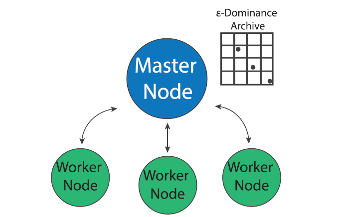
Figure 1: The Master Worker implementation of the Borg MOEA. (Figure from Salazar et al., 2017)

MOEA search is “embarrassingly parallel” since the evaluation of each candidate solution can be done independently of other solutions in a population (Cantu-Paz, 2000). The master-worker paradigm of MOEA parallelization, which has been in use since early days of evolutionary algorithms (Grefenstette, 1981), utilizes this property to parallelize search. In the master worker implementation of Borg in a system of P processors, one processor is designated as the “master” and P-1 processors are designated as “workers”. The master processor runs the serial version of the Borg MOEA but instead of evaluating candidate solution, it sends the decision variables to an available worker which evaluates the problem with the given decision variables and sends the evaluated objectives and constraints back to the master processor.

Most MOEAs are generational, meaning that they evolve a population in distinct stages known as generations (Coello Coello et al., 2007). During one generation, the algorithm evolves the population to produce offspring, evaluates the offspring and then adds them back into the population (methods for replacement of existing members vary according to the MOEA). When run in parallel, generational MOEAs must evaluate every solution in a generation before beginning evaluation of the next generation. Since these algorithms need to synchronize function evaluations within a generation, they are known as synchronous MOEAs. Figure 2, from Hadka et al., (2013b), shows a timeline of events for a typical synchronous MOEA. Algorithmic time (TA) represents the time it takes the master processor to perform the serial components of the MOEA. Function evaluation time (TF) is the the time it takes to evaluate one offspring and communication time (TC) is the time it takes to pass information to and from worker nodes. The vertical dotted lines in Figure 2 represent the start of each new generation. Note the periods of idle time that each worker node experiences while it waits for the algorithm to perform serial calculations and communicate. If the function evaluation time is not constant across all nodes, this idle time can increase as the algorithm waits for all solutions in the generation to be evaluated.

Figure 2: Diagram of a synchronous MOEA. Tc represents communication time, TA represents algorithmic time and TF represents function evaluation time. (Figure from Hadka et al., 2013b).

The Borg MOEA is not generational but rather a steady-state algorithm. As soon as an offspring is evaluated by a worker and returned to the master, the next offspring is immediately sent to the worker for evaluation. This is accomplished through use of a queue, for details of Borg’s queuing process see Hadka and Reed, (2015). Since Borg is not bound by the need to synchronize function evaluations within generations, it is known as an asynchronous MOEA. Figure 3, from Hadka et al., (2013b), shows a timeline of a events for a typical Borg run. Note that the idle time has been shifted from the workers to the master processor. When the algorithm is parallelized across a large number of cores, the decreased idle time for each worker has the potential to greatly increase the algorithm’s parallel efficiency. Furthermore, if function evaluation times are heterogeneous, the algorithm is not bottlenecked by slow evaluations as generational MOEAs are.

Figure 3: Diagram of an asynchronous MOEA. Tc represents communication time, TA represents algorithmic time and TF represents function evaluation time. (Figure from Hadka et al., 2013b).

While the master-worker implementation of the Borg MOEA is an efficient means of parallelizing function evaluations, the search algorithm’s search dynamics remain the same as the serial version and as the number of processors increases, the search may suffer from communication bottlenecks. The multi-master implementation of the Borg MOEA uses parallelization to not only improve the efficiency of function evaluations but also improve the quality of the multi-objective search.

Multi-Master Borg

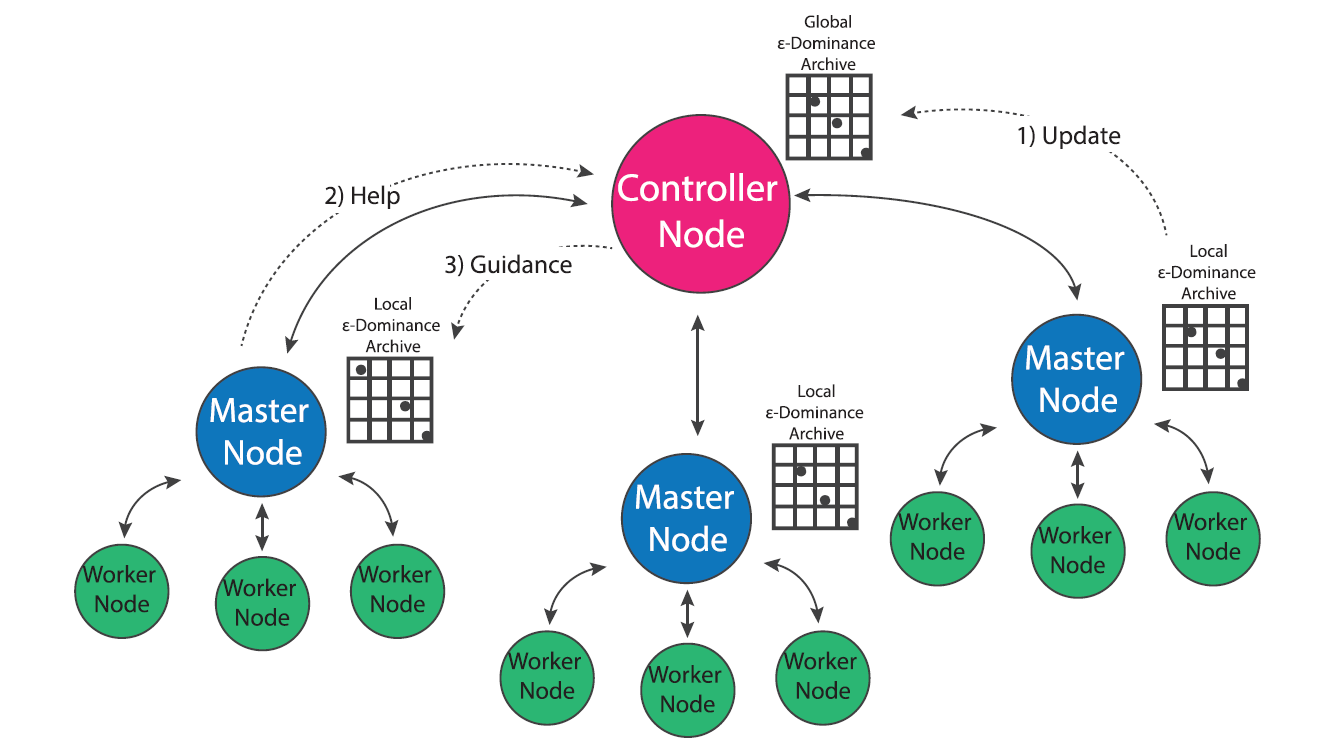
Figure 4: The multi-master implementation of the Borg MOEA. (Figure from Salazar et al., 2017)

In population genetics, the “island model” considers distinct populations that evolve independently but periodically interbreed via migration events that occur over the course of the evolutionary process (Cantu-Paz, 2000). Two independent populations may evolve very different survival strategies based on the conditions of their environment (i.e. locally optimal strategies). Offspring of migration events that combine two distinct populations have the potential to combine the strengths developed by both groups. This concept has been utilized in the development of multi-population evolutionary algorithms (also called multi-deme algorithms in literature) that evolve multiple populations in parallel and occasionally exchange individuals via migration events (Cantu-Paz, 2000). Since MOEAs are inherently stochastic algorithms that are influenced by their initial populations, evolving multiple populations in parallel has the potential to improve the efficiency, quality and reliability of search results (Hadka and Reed, 2015; Salazar et al., 2017). Hybrid parallelization schemes that utilize multiple versions of master-worker MOEAs may further improve the efficiency of multi-population search (Cantu-Paz, 2000). However, the use of a multi-population MOEA requires the specification of parameters such as the number of islands, number of processors per island and migration policy that whose ideal values are not apparent prior to search.

The multi-master implementation of the Borg MOEA is a hybrid parallelization of the MOEA that seeks to generalize the algorithm’s ease of use and auto-adaptivity while maximizing its parallel efficiency on HPC architectures (Hadka and Reed, 2015). In the multi-master implementation, multiple versions of the master-worker MOEA are run in parallel, and an additional processor is designated as the “controller”. Each master maintains its own epsilon dominance archive and operator probabilities, but regulatory updates its progress with the controller which maintains a global epsilon dominance archive and global operator probabilities. If a master processor detects search stagnation that it is not able to overcome via Borg’s automatic restarts, it requests guidance from the controller node which seeds the master with the contents of the global epsilon dominance archive and operator probabilities. This guidance system insures that migration events between populations only occurs when one population is struggling and only consists of globally non-dominated solutions. Borg’s adaptive population sizing ensures the injected population is resized appropriately given the global search state.

The use of multiple-populations presents an opportunity for the algorithm to improve the sampling of the initial population. The serial and master-worker implementations of Borg generate the initial population by sampling decision variables uniformly at random from their bounds, which has the potential to introduce random bias into the initial search population (Hadka and Reed, 2015). In the multi-master implementation of Borg, the controller node first generates a latin hypercube sample of the decision variables, then distributes these samples between masters uniformly at random. This initial sampling strategy adds some additional overhead to the algorithm’s startup, but ensures that globally the algorithm starts with a well-distributed, diverse set of initial solutions which can help avoid preconvergence (Hadka and Reed, 2015).

Conclusion

This post has reviewed two parallel implementations of the Borg MOEA. The next post in this series will discuss how to evaluate parallel performance of a MOEA in terms of search efficiency, quality and reliability. I’ll review recent literature comparing performance of master-worker and multi-master Borg and discuss how to determine which implementation is appropriate for a given problem.

References

Cantu-Paz, E. (2000). Efficient and accurate parallel genetic algorithms (Vol. 1). Springer Science & Business Media.

Hadka, D., Reed, P. M., & Simpson, T. W. (2012). Diagnostic assessment of the Borg MOEA for many-objective product family design problems. 2012 IEEE Congress on Evolutionary Computation (pp. 1-10). IEEE.

Hadka, D., & Reed, P. (2013a). Borg: An auto-adaptive many-objective evolutionary computing framework. Evolutionary computation21(2), 231-259.

Hadka, D., Madduri, K., & Reed, P. (2013b). Scalability analysis of the asynchronous, master-slave borg multiobjective evolutionary algorithm. In 2013 IEEE International Symposium on Parallel & Distributed Processing, Workshops and Phd Forum (pp. 425-434). IEEE.

Hadka, D., & Reed, P. (2015). Large-scale parallelization of the Borg multiobjective evolutionary algorithm to enhance the management of complex environmental systems. Environmental Modelling & Software69, 353-369.

Salazar, J. Z., Reed, P. M., Quinn, J. D., Giuliani, M., & Castelletti, A. (2017). Balancing exploration, uncertainty and computational demands in many objective reservoir optimization. Advances in water resources109, 196-210.