In Parallel Programming Part 1, I introduced a number of basic OpenMP directives and constructs, as well as provided a quick guide to high-performance computing (HPC) terminology. In Part 2 (aka this post), we will apply some of the constructs previously learned to execute a few OpenMP examples. We will also view an example of incorrect use of OpenMP constructs and its implications.
TheCube Cluster Setup
Before we begin, there are a couple of steps to ensure that we will be able to run C++ code on the Cube. First, check the default version of the C++ compiler. This compiler essentially transforms your code into an executable file that can be easily understood and implemented by the Cube. You can do this by entering
g++ --version
into your command line. You should see that the Cube has G++ version 8.3.0 installed, as shown below.
Now, create two files:
openmp-demo-print.cpp this is the file where we will perform a print demo to show how tasks are distributed between threads
openmp-demo-access.cpp this file will demonstrate the importance of synchronization and the implications if proper synchronization is not implemented
Example 1: Hello from Threads
Open the openmp-demo-print.cpp file, and copy and paste the following code into it:
#include <iostream>
#include <omp.h>
#include <stdio.h>

int main() {

    int num_threads = omp_get_max_threads(); // get max number of threads available on the Cube
    omp_set_num_threads(num_threads);

    printf("The CUBE has %d threads.\n", num_threads);


    #pragma omp parallel
    {
        int thread_id = omp_get_thread_num();
        printf("Hello from thread num %d\n", thread_id);
    }

    printf("Thread numbers written to file successfully. \n");

    return 0;
}
Here is what the code is doing:
Lines 1 to 3 are the libraries that need to be included in this script to enable the use of OpenMP constructs and printing to the command line.
In main() on Lines 7 and 8, we first get the maximum number of threads that the Cube has available on one node and assign it to the num_threads variable. We then set the number of threads we want to use.
Next, we declare a parallel section using #pragma omp parallel beginning on Line 13. In this section, we are assigning the printf() function to each of the num_threads threads that we have set on Line 8. Here, each thread is now executing the printf() function independently of each other. Note that the threads are under no obligation to you to execute their tasks in ascending order.
Finally, we end the call to main() by returning 0
Be sure to first save this file. Once you have done this, enter the following into your command line:
This tells the system to compile openmp-demo-print.cpp and create an executable object using the same file name. Next, in the command line, enter:
./openmp-demo-print
You should see the following (or some version of it) appear in your command line:
Notice that the threads are all being printed out of order. This demonstrates that each thread takes a different amount of time to complete its task. If you re-run the following script, you will find that the order of threads that are printed out would have changed, showing that there is a degree of uncertainty associated with the amount of time they each require. This has implications for the order in which threads read, write, and access data, which will be demonstrated in the next example.
Example 2: Who’s (seg)Fault Is It?
In this example, we will first execute a script that stores each thread number ID into an array. Each thread then accesses its ID and prints it out into a text file called access-demo.txt. See the implementation below:
#include <iostream>
#include <omp.h>
#include <vector>

using namespace std;

void parallel_access_demo() {
    vector<int> data;
    int num_threads = omp_get_max_threads();

    // Parallel region for appending elements to the vector
    #pragma omp parallel for
    for (int i = 0; i < num_threads; ++i) {
        // Append the thread ID to the vector
        data.push_back(omp_get_thread_num()); // Potential race condition here
    }
}

int main() {
    // Execute parallel access demo
    parallel_access_demo();
    printf("Code ran successfully. \n");

    return 0;
}
As per the usual, here’s what’s going down:
After including the necessary libraries, we use include namespace std on Line 5 so that we can more easily print text without having to used std:: every time we attempt to write a statement to the output file
Starting on Line 7, we write a simple parallel_access_demo() function that does the following:
Initialize a vector of integers very creatively called data
Get the maximum number of threads available per node on the Cube
Declare a parallel for region where we iterate through all threads and push_back the thread ID number into the data vector
Finally, we execute this function in main() beginning Line 19.
If you execute this using a similar process shown in Example 1, you should see the following output in your command line:
Congratulations – you just encountered your first segmentation fault! Not to worry – this is by design. Take a few minutes to review the code above to identify why this might be the case.
Notice Line 15. Where, each thread is attempting to insert a new integer into the data vector. Since push_back() is being called in a parallel region, this means that multiple threads are attempting to modify data simultaneously. This will result in a race condition, where the size of data is changing unpredictably. There is a pretty simple fix to this, where we add a #pragma omp criticalbefore Line 15.
As mentioned in Part 1, #pragma omp critical ensures that each thread executes its task one at a time, and not all at once. It essentially serializes a portion of the parallel for loop and prevents race conditions by ensuring that the size of data changes in a predictable and controlled manner. An alternative would be to declare #pragma omp single in place of #pragma omp parallel foron Line 12. This essentially delegates the following for-loop to a single thread, forcing the loop to be completed in serial. Both of these options will result in the blissful outcome of
Summary
In this post, I introduced two examples to demonstrate the use of OpenMP constructs. In Example 1, I demonstrated a parallel printing task to show that threads do not all complete their tasks at the same time. Example 2 showed how the lack of synchronization can lead to segmentation faults due to race conditions, and two methods to remedy this. In Part 3, I will introduce GPU programming using the Python PyTorch library and Google Colaboratory cloud infrastructure. Until then, happy coding!
Hybrid parallelization is often used when performing noisy simulation-optimization on high-performance computing clusters. One common technique is to divide the available CPUs into a smaller number of “tasks”, each of which uses its subset of CPUs to assess the performance of candidate solutions through parallel evaluation of multiple scenarios. In this post, I will demonstrate how to use Python’s Multiprocessing module to set up a hybrid parallelization scheme with the Borg MOEA, and explore the resulting tradeoff between efficiency and learning rate in order to better understand when one should (and should not) implement such a scheme.
This post will bring together and build upon several previous posts on this blog, including (1) this demonstration by Andrew Dircks for how to use the Borg MOEA’s Python wrapper to optimize multi-objective simulations written in Python, using the Lake Problem as example; (2) this explanation of the Borg MOEA’s hybrid parallelization strategies by David Gold; and (3) this post by Bernardo Trindade on parallelizing Monte Carlo evaluations using Python and C/C++. The present post will give a brief overview of these topics in order to show how they can be brought together, but the reader is referred to the posts above for more detail on any of these topics.
Why hybrid parallelization?
As a motivating example, consider a complex water resources simulation model that takes 10 minutes to run a 30 year simulation. We want to explore the potential for new infrastructure investments to improve multiple objectives such as water supply reliability, cost, etc. We will try to discover high-performing solutions using an MOEA. To account for uncertainty, each candidate investment will be evaluated in 48 different stochastic scenarios.
Given the expense of our simulation model, this will be a major computational challenge. If we evaluate 20,000 candidate solutions (which is quite low compared to other studies), the total run time will be 20000 * 48 * 10 minutes = 6,667 days. Clearly, we cannot afford to run this serially on a laptop. If we have access to a computer cluster, we can parallelize the MOEA search and speed things up drastically. For example, with an XSEDE allocation on TACC Stampede2, I can run jobs with up to 128 Skylake nodes, each of which has 48 CPU, for a total of 6144 CPU per job. With this setup, we could finish the same experiment in ~1.1 days.
With the simplest possible parallelization strategy, we have a single CPU as the “Master” for the Borg MOEA, and 6143 CPU running individual function evaluations (FE). Each FE is allocated a single CPU, which runs 48 stochastic simulations in serial (i.e., there is no hybrid parallelization taking place). At the other extreme, I could set the MOEA to run with an entire node per “task”. This would allocate a full node to the Borg Master process, plus 127 nodes running individual FEs. Each FE would distribute its 48 stochastic simulations across its 48 CPUs in parallel. Thus, we are running fewer concurrent FEs (127 vs. 6143), but each finishes much faster (10 minutes vs. 480 minutes). In between these two extremes, there are intermediate parallelization schemes that allocate 2, 3, 4, 6, 8, 12, 16, or 24 CPU per task (Table 1).
So how to choose a parallelization strategy? The first thing to consider is efficiency. In theory, the scheme without hybrid parallelization (1 CPU per task) is the most efficient, since it allocates only one CPU to the Borg Master process, allowing for 6143 CPU to be simultaneously performing simulations. The 48 CPU/task scheme, on the other hand, allocates an entire node to the Borg Master (even though it only needs a single CPU to perform its duties), so that only 127*48=6096 CPU are running simulations at a given time. Thus, it should be ~1% slower in theory. However, in practice, a variety of factors such as communication or I/O bottlenecks can change this behavior (see below), so it is important to run tests on your particular machine.
If the hybrid parallelization scheme is slower, why should we even consider it? The key point is the increased potential for “learning” within the MOEA loop. Remember that the 1 CPU/task scheme has 6143 FE running concurrently, while the 48 CPU/task scheme has 127 FE. This means that the former will only have approximately 20000/6143=3.3 “generations,” while the latter will have 20000/127=157.5 generations*. Put another way, each FE will take 480 minutes (30% of total 1.1 days) to complete for the 1 CPU/task scheme, compared to 10 minutes (0.6% of total) for the 48 CPU/task scheme. The latter thus provides a more continuous stream of information to the MOEA Master, and therefore many more opportunities for the MOEA to learn what types of solutions are successful through iterative trial and error.
*Note: The Borg MOEA is a steady-state algorithm rather than a generational algorithm, so I use the term “generation” loosely to refer to the number of FE that each task will complete. See Dave Gold’s blog post on the Borg MOEA’s parallelization for more details on generational vs. steady-state algorithms. Note that for this post, I am using the master-worker variant of the Borg MOEA.
Function evaluations (FE)
Total CPU
Tasks/node
CPU/task
Concurrent FE
Generations
20000
6144
48
1
6143
3.3
20000
6144
24
2
3071
6.5
20000
6144
16
3
2047
9.8
20000
6144
12
4
1535
13.0
20000
6144
8
6
1023
19.6
20000
6144
6
8
767
26.1
20000
6144
4
12
511
39.1
20000
6144
3
16
383
52.2
20000
6144
2
24
255
78.4
20000
6144
1
48
127
157.5
Table 1: Scaling of concurrent function evaluations and generations for different hybrid parallelization schemes, using 128 Skylake nodes (48 CPU each) on Stampede2.
A simple example: hybrid parallelization of the Lake Problem in Python
Above, I have outlined a purely theoretical tradeoff between efficiency and algorithmic learning. How does this tradeoff play out in practice? What type of hybrid scheme is “best”? I will now explore these questions in more detail using a smaller-scale example. The Lake Problem is a popular example for demonstrating concepts such as non-linear dynamics, deep uncertainty, and adaptive multi-objective control; a search for “Lake Problem” on the Water Programming Blog returns many results (I stopped counting at 30). In this problem, the decision-maker is tasked with designing a regulatory policy that balances the economic benefits of phosphorus with its environmental risks, given the large uncertainty in the complex dynamics that govern lake pollution concentrations over time. In a 2017 article in Environmental Modelling & Software, Julie Quinn demonstrated the merits of Evolutionary Multi-Objective Direct Policy Search (EMODPS) for developing control policies that adaptively update phosphorus releases based on evolving conditions (e.g., current lake concentration).
A Python version of the EMODPS Lake Problem was introduced along with a Python wrapper for the Borg MOEA in this blog post by Andrew Dircks. Additionally, this post by Bernardo Trindade demonstrates how to parallelize Monte Carlo ensembles in Python as well as C/C++. For the present example, I combined aspects of these two posts, in order to parallelize the Monte Carlo evaluations within each function evaluation, using the Multiprocessing module in Python. For this blog post, I will highlight a few of the important differences relative to the non-parallel version of the problem in Andrew Dircks’ blog post, but the interested reader is referred to these previous two post for more detail. All code used to produce these results can be found in this GitHub repository.
The lake_mp.py file specifies the analysis that the Borg MOEA should run for each function evaluation – we will evaluate each candidate operating policy using an ensemble of 48 simulations, each of which uses a different 100-year stochastic realization of hydrology. This ensemble will be divided among a smaller number of CPUs (say, 16) assigned to each function evaluation. Thus, we will have to set up our code a bit differently than in the serial version. First, consider the overall “problem” function which is called by the Borg Master. Within this function, we can set up shared arrays for each objective. The Array class from the multiprocessing module allows for thread-safe access to the same memory array from multiple CPUs. Note that this module requires shared memory (i.e., the CPUs must be on the same node). If you want to share memory across multiple nodes, you will need to use the mpi4py module, rather than multiprocessing.
from multiprocessing import Process, Array
# create shared memory arrays which each process can access/write.
discounted_benefit = Array('d', nSamples)
yrs_inertia_met = Array('i',  nSamples)
yrs_Pcrit_met = Array('i', nSamples)
average_annual_P = Array('d', nSamples*nYears)
Now we need to figure out which simulations should be performed by each CPU, and dispatch those simulations using the Process class from the multiprocessing module.
# assign MC runs to different processes
nbase = int(nSamples / nProcesses)
remainder = nSamples - nProcesses * nbase
start = 0
shared_processes = []
for proc in range(nProcesses):
    nTrials = nbase if proc >= remainder else nbase + 1
    stop = start + nTrials
    p = Process(target=dispatch_MC_to_procs, args=(proc, start, stop, discounted_benefit, yrs_inertia_met, yrs_Pcrit_met, average_annual_P, natFlow, b, q, critical_threshold, C, R, newW))

    shared_processes.append(p)
    start = stop

# start processes
for sp in shared_processes:
    sp.start()

# wait for all processes to finish
for sp in shared_processes:
    sp.join()
The “args” given to the Process function contains information needed by the individual CPUs, including the shared memory arrays. Once we have appended the processes for each CPU, we start them, and then wait for all processes to finish (“join”).
The “target” in the Process function tells each CPU which subset of Monte Carlo samples to evaluate, and runs the individual evaluations in a loop:
#Sub problem to dispatch MC samples from individual processes
def dispatch_MC_to_procs(proc, start, stop, discounted_benefit, yrs_inertia_met, yrs_Pcrit_met, average_annual_P, natFlow, b, q, critical_threshold, C, R, newW):
    lake_state = np.zeros([nYears + 1])
    Y = np.zeros([nYears])
    for s in range(start, stop):
        LakeProblem_singleMC(s, discounted_benefit, yrs_inertia_met, yrs_Pcrit_met, average_annual_P, lake_state, natFlow[s, :], Y, b, q, critical_threshold, C, R, newW)
Within the loop, we call LakeProblem_singleMC to run each Monte Carlo evaluation. After running the simulation, this function can store its sub-objectives in the shared arrays:
# fill in results for MC trial in shared memory arrays, based on index of this MC sample (s)
average_annual_P[(s*nYears):((s+1)*nYears)] = lake_state[1:]
discounted_benefit[s] = db
yrs_inertia_met[s] = yim
yrs_Pcrit_met[s] = yPm
Finally, back in the main “problem” function, we can evaluate the objectives by aggregating over the shared memory arrays:
# Calculate minimization objectives (defined in comments at beginning of file)
objs[0] = -1 * np.mean(discounted_benefit)  #average economic benefit
objs[1] = np.max(np.mean(np.reshape(average_annual_P, (nSamples, nYears)), axis=0))  #minimize the max average annual P concentration
objs[2] = -1 * np.sum(yrs_inertia_met) / ((nYears - 1) * nSamples)  #average percent of transitions meeting inertia thershold
objs[3] = -1 * np.sum(yrs_Pcrit_met) / (nYears * nSamples)  #average reliability
constrs[0] = max(0.0, reliability_threshold - (-1 * objs[3]))

time.sleep(slp)
In the last line, I add a half-second sleep after each function evaluation in order to help this example better mimic the behavior of the much slower motivating problem at the beginning of this post. Without the sleep, the Lake Problem is much faster than larger simulation codes, and therefore could exhibit additional I/O and/or master-worker interaction bottlenecks.
Again, the interested reader is referred to the GitHub repository, as well as Andrew Dircks’ original Lake Problem blog post, for more details on how these code snippets fit into the broader program.
This experiment is run on the Cube cluster at Cornell University, using 12 nodes of 16 CPU each. I tested 5 different hybrid parallelization schemes, from 1 to 16 CPU per task (Table 2). Each formulation is run for 5 seeds to account for the random dynamics of evolutionary algorithms. For this experiment, I will show results through 800 function evaluations. Although this is much smaller than the standard practice, this short experiment allows us to mimic the behavior of the much larger experiment introduced at the beginning of this post (compare the number of Generations in Tables 1 & 2).
Function evaluations (FE)
Total CPU
Tasks/node
CPU/task
Concurrent FE
Generations
800
192
16
1
191
4.2
800
192
8
2
95
8.4
800
192
4
4
47
17.0
800
192
2
8
23
34.8
800
192
1
16
11
72.7
Table 2: Scaling of concurrent function evaluations and generations for different hybrid parallelization schemes, using 12 nodes (16 CPU each) on TheCube.
How do different parallelization schemes compare?
Figure 1 shows the performance of the 1 & 16 CPU/task schemes, in terms of hypervolume of the approximate Pareto set. The hybrid parallelization scheme (16 CPU/task) is found to outperform the serial scheme (1 CPU/task). In general across the five seeds, the parallelized scheme is found to improve more quickly and to reach a higher overall hypervolume after 800 FE. The intermediate parallelization schemes (2, 4, & 8 CPU/task) are found to perform similarly to the 16 CPU/task (see GitHub repository for figures)
Figure 1: Hypervolume vs. number of function evaluations for parallelization schemes with 1 and 16 CPU per function evaluation.
Figure 2 shows the number of completed function evaluations over time, which helps illuminate the source of this advantage. The serial formulation shows a staircase pattern: large chunks of time with no progress, followed by short bursts with many FE finishing all at once. Overall, the FE arrive in 5 major bursts (with the last smaller than the rest), at approximately 25, 50, 75, 100, and 125 seconds. As we move to 2, 4, 8, and 16 CPU/task, the number of “stairs” is seen to double each time, so that the 16 CPU/task scheme almost approximates a straight line. These patterns are consistent with the generational pattern shown in Table 2.
Figure 2: Runtime vs. number of function evaluations for parallelization schemes with 1, 2, 4, 8, and 16 CPU per function evaluation.
So why does this matter? Elitist evolutionary algorithms use the relative performance of past evaluations to influence the random generation of new candidate solutions. Because a hybrid parallelization strategy evaluates fewer solutions concurrently and has more “generations” of information, there will be more ability to learn over the course of the optimization. For example, with the serial scheme, the first generation of 191 candidate solutions is randomly generated with no prior information. The 16 CPU/task scheme, on the other hand, only produces 11 solutions in the first generation, and has had ~17 generations worth of learning by the time it reaches 191 FE.
Additionally, the Borg MOEA has a variety of other auto-adaptive features that can improve the performance of the search process over the course of a single run (see Hadka & Reed, 2013). For example, Borg has six different recombination operators that can be used to mate and mutate previously evaluated solutions in order to generate new candidates for evaluation. The MOEA adaptively updates these selection probabilities in favor of the operators which have been most successful at producing successful offspring. The hybrid parallelization allows these probabilities to be adapted earlier and more regularly due to the more continuous accumulation of information (Figure 3). This can improve the performance of the MOEA.
Figure 3: Operator probabilities vs number of function evaluations (NFE) for parallelization schemes with 1 and 16 CPU per function evaluation. The subplots represent the auto-adaptive selection probabilities for the six recombination operators used by the Borg MOEA: differential evolution (DE), parent-centric crossover (PCX), simulated binary crossover (SBX), simplex crossover (PCX), uniform mutation (UM), and unimodal normal distribution crossover (UNDX).
What happens in longer runs?
At this point, it may seem that hybrid parallelization is always beneficial, since it can increase the algorithm’s adaptability (Figure 3) and improve performance (Figure 1) for a fairly negligible computational cost (Figure 2). However, the experiments in Tables 1 & 2 are very constrained in terms of the number of generations that are run. In most contexts, we will have more function evaluations and/or fewer nodes, so that the ratio of nodes to FE is much smaller and thus the number of generations is much larger. In these situations, do the advantages of hybrid parallelization hold up?
Figure 4 shows the results of a longer experiment, which is identical to above except for its use of 10,000 FE rather than 800 FE. Over the longer experiment, the advantage of the parallelized scheme (16 CPU/FE) is found to diminish, with random seed variability becoming dominant. With more generations, the differences between the two schemes seems to fade.
Figure 4: Same as Figure 1, but for a longer experiment of 10,000 function evaluations.
Figure 5 shows the evolution of the recombination operator selection probabilities over the longer experiment. The serial scheme still lags in terms of adaptation speed, but by the end of the experiment, the two formulations have very similar behavior.
Figure 5: Same as Figure 3, but for a longer experiment of 10,000 function evaluations.
Lastly, Figure 6 shows the runtime as a function of FEs for the two formulations. The parallelized scheme takes approximately 15% longer than the serial scheme. We can compare this to the theoretical slowdown based on the Borg Master overhead: the 16 CPU/task scheme runs 11 concurrent FE, each using 16 CPU, for a total of 176 CPU, while the serial version runs 191 concurrent FE, each using 1 CPU. 191 is 9% larger than 176. The difference between 15% and 9% indicates additional bottlenecks, such as writing to the shared array. This overhead may vary based on the characteristics of the cluster and the computational experiment, so testing should be performed prior to running any large experiment.
Figure 6: Same as Figure 2, but for a longer experiment of 10,000 function evaluations.
Given all this information, what to do? Should you use hybrid parallelization for your function evaluations? The answer, unsatisfyingly, is “it depends.” The most important factor to consider is the number of generations for your optimization, calculated as the total number of FE divided by the number of concurrent FE. If this number is relatively high (say, >10-20), then you may be better off sticking with serial FEs in order to improve efficiency. If the number of generations is small, it may be worthwhile to introduce hybrid parallelization in order to stimulate adaptive learning within the MOEA. Where to draw the line between these two poles will likely to vary based on a number of factors, including the number of nodes you are using, the computational architecture of the cluster, the runtime of each function evaluation, and the difficulty of the optimization problem, so testing is recommended to decide what to do in any given scenario.
This post will introduce basic concepts regarding the parallelization of the Borg Multiobjective Evolutionary Algorithm (Borg MOEA). In this post I’ll assume the reader is familiar with the basic architecture of the Borg MOEA, if you’re unfamiliar with the algorithm or would like a refresher, see Hadka and Reed, (2013a) before reading further.
Parallelization Basics
Before we go into parallization of Borg, let’s quickly define some terminology. Modern High Performance Computing (HPC) resources are usually comprised of many multi-core processors, each consisting of two or more processing cores. For this post, I’ll refer to an individual processing core as a “processor”. Parallel computing refers to programs that utilize multiple processors to simultaneously perform operations that would otherwise be performed in serial on a single processor.
Parallel computing can be accomplished using either “distributed” or “shared” memory methods. Shared memory methods consist of parallelizing tasks across a group of processors that all read and write from the same memory space. In distributed memory parallelization, each processor maintains its own private memory and data is usually passed between processors using a message passing interface (MPI) library. Parallel Borg applications are coded using distributed memory parallelization, though it’s important to note that it’s possible to parallelize the simulation model that is coupled with Borg using shared memory parallelization. For additional reading on parallelization concepts see Bernardo’s post from April and Barney’s posts from 2017.
Hadka et al., (2012) showed that the quality of search results discovered by the Borg MOEA is strongly dependent on the number of function evaluations (NFE) performed in an optimization run. Efficient parallelization of search on HPC resources can allow not only for the search to be performed “faster” but also may allow more NFE to be run, potentially improving the quality of the final approximation of the Pareto front. Parallelization also offers opportunities to improve the search dynamics of the MOEA, improving the reliability and efficiency of multi-objective search (Hadka and Reed, 2015; Salazar et al., 2017).
Below I’ll discuss two parallel implementations of the Borg MOEA, a simple master-worker implementation to parallelize function evaluations across multiple processors and an advanced hybrid multi-population implementation that improves search dynamics and is scalable Petascale HPC resources.
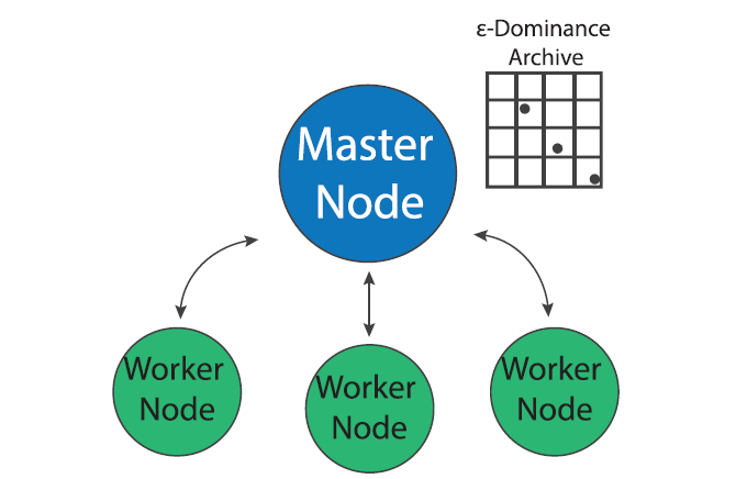
Master-worker Borg
Figure 1: The Master Worker implementation of the Borg MOEA. (Figure from Salazar et al., 2017)
MOEA search is “embarrassingly parallel” since the evaluation of each candidate solution can be done independently of other solutions in a population (Cantu-Paz, 2000). The master-worker paradigm of MOEA parallelization, which has been in use since early days of evolutionary algorithms (Grefenstette, 1981), utilizes this property to parallelize search. In the master worker implementation of Borg in a system of P processors, one processor is designated as the “master” and P-1 processors are designated as “workers”. The master processor runs the serial version of the Borg MOEA but instead of evaluating candidate solution, it sends the decision variables to an available worker which evaluates the problem with the given decision variables and sends the evaluated objectives and constraints back to the master processor.
Most MOEAs are generational, meaning that they evolve a population in distinct stages known as generations (Coello Coello et al., 2007). During one generation, the algorithm evolves the population to produce offspring, evaluates the offspring and then adds them back into the population (methods for replacement of existing members vary according to the MOEA). When run in parallel, generational MOEAs must evaluate every solution in a generation before beginning evaluation of the next generation. Since these algorithms need to synchronize function evaluations within a generation, they are known as synchronous MOEAs. Figure 2, from Hadka et al., (2013b), shows a timeline of events for a typical synchronous MOEA. Algorithmic time (TA) represents the time it takes the master processor to perform the serial components of the MOEA. Function evaluation time (TF) is the the time it takes to evaluate one offspring and communication time (TC) is the time it takes to pass information to and from worker nodes. The vertical dotted lines in Figure 2 represent the start of each new generation. Note the periods of idle time that each worker node experiences while it waits for the algorithm to perform serial calculations and communicate. If the function evaluation time is not constant across all nodes, this idle time can increase as the algorithm waits for all solutions in the generation to be evaluated.
Figure 2: Diagram of a synchronous MOEA. Tc represents communication time, TA represents algorithmic time and TF represents function evaluation time. (Figure from Hadka et al., 2013b).
The Borg MOEA is not generational but rather a steady-state algorithm. As soon as an offspring is evaluated by a worker and returned to the master, the next offspring is immediately sent to the worker for evaluation. This is accomplished through use of a queue, for details of Borg’s queuing process see Hadka and Reed, (2015). Since Borg is not bound by the need to synchronize function evaluations within generations, it is known as an asynchronous MOEA. Figure 3, from Hadka et al., (2013b), shows a timeline of a events for a typical Borg run. Note that the idle time has been shifted from the workers to the master processor. When the algorithm is parallelized across a large number of cores, the decreased idle time for each worker has the potential to greatly increase the algorithm’s parallel efficiency. Furthermore, if function evaluation times are heterogeneous, the algorithm is not bottlenecked by slow evaluations as generational MOEAs are.
Figure 3: Diagram of an asynchronous MOEA. Tc represents communication time, TA represents algorithmic time and TF represents function evaluation time. (Figure from Hadka et al., 2013b).
While the master-worker implementation of the Borg MOEA is an efficient means of parallelizing function evaluations, the search algorithm’s search dynamics remain the same as the serial version and as the number of processors increases, the search may suffer from communication bottlenecks. The multi-master implementation of the Borg MOEA uses parallelization to not only improve the efficiency of function evaluations but also improve the quality of the multi-objective search.
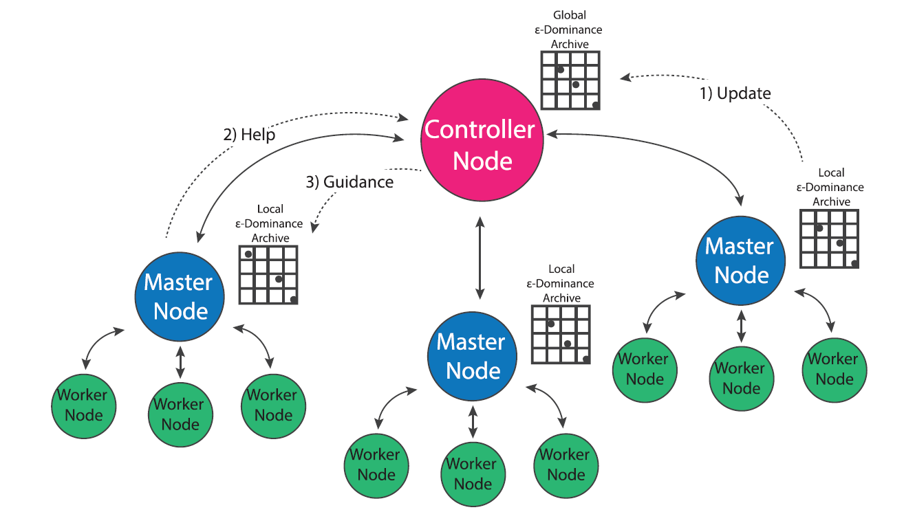
Multi-Master Borg
Figure 4: The multi-master implementation of the Borg MOEA. (Figure from Salazar et al., 2017)
In population genetics, the “island model” considers distinct populations that evolve independently but periodically interbreed via migration events that occur over the course of the evolutionary process (Cantu-Paz, 2000). Two independent populations may evolve very different survival strategies based on the conditions of their environment (i.e. locally optimal strategies). Offspring of migration events that combine two distinct populations have the potential to combine the strengths developed by both groups. This concept has been utilized in the development of multi-population evolutionary algorithms (also called multi-deme algorithms in literature) that evolve multiple populations in parallel and occasionally exchange individuals via migration events (Cantu-Paz, 2000). Since MOEAs are inherently stochastic algorithms that are influenced by their initial populations, evolving multiple populations in parallel has the potential to improve the efficiency, quality and reliability of search results (Hadka and Reed, 2015; Salazar et al., 2017). Hybrid parallelization schemes that utilize multiple versions of master-worker MOEAs may further improve the efficiency of multi-population search (Cantu-Paz, 2000). However, the use of a multi-population MOEA requires the specification of parameters such as the number of islands, number of processors per island and migration policy that whose ideal values are not apparent prior to search.
The multi-master implementation of the Borg MOEA is a hybrid parallelization of the MOEA that seeks to generalize the algorithm’s ease of use and auto-adaptivity while maximizing its parallel efficiency on HPC architectures (Hadka and Reed, 2015). In the multi-master implementation, multiple versions of the master-worker MOEA are run in parallel, and an additional processor is designated as the “controller”. Each master maintains its own epsilon dominance archive and operator probabilities, but regulatory updates its progress with the controller which maintains a global epsilon dominance archive and global operator probabilities. If a master processor detects search stagnation that it is not able to overcome via Borg’s automatic restarts, it requests guidance from the controller node which seeds the master with the contents of the global epsilon dominance archive and operator probabilities. This guidance system insures that migration events between populations only occurs when one population is struggling and only consists of globally non-dominated solutions. Borg’s adaptive population sizing ensures the injected population is resized appropriately given the global search state.
The use of multiple-populations presents an opportunity for the algorithm to improve the sampling of the initial population. The serial and master-worker implementations of Borg generate the initial population by sampling decision variables uniformly at random from their bounds, which has the potential to introduce random bias into the initial search population (Hadka and Reed, 2015). In the multi-master implementation of Borg, the controller node first generates a latin hypercube sample of the decision variables, then distributes these samples between masters uniformly at random. This initial sampling strategy adds some additional overhead to the algorithm’s startup, but ensures that globally the algorithm starts with a well-distributed, diverse set of initial solutions which can help avoid preconvergence (Hadka and Reed, 2015).
Conclusion
This post has reviewed two parallel implementations of the Borg MOEA. The next post in this series will discuss how to evaluate parallel performance of a MOEA in terms of search efficiency, quality and reliability. I’ll review recent literature comparing performance of master-worker and multi-master Borg and discuss how to determine which implementation is appropriate for a given problem.
References
Cantu-Paz, E. (2000). Efficient and accurate parallel genetic algorithms (Vol. 1). Springer Science & Business Media.
Hadka, D., Reed, P. M., & Simpson, T. W. (2012). Diagnostic assessment of the Borg MOEA for many-objective product family design problems. 2012 IEEE Congress on Evolutionary Computation (pp. 1-10). IEEE.
Hadka, D., & Reed, P. (2013a). Borg: An auto-adaptive many-objective evolutionary computing framework. Evolutionary computation, 21(2), 231-259.
Hadka, D., Madduri, K., & Reed, P. (2013b). Scalability analysis of the asynchronous, master-slave borg multiobjective evolutionary algorithm. In 2013 IEEE International Symposium on Parallel & Distributed Processing, Workshops and Phd Forum (pp. 425-434). IEEE.
Hadka, D., & Reed, P. (2015). Large-scale parallelization of the Borg multiobjective evolutionary algorithm to enhance the management of complex environmental systems. Environmental Modelling & Software, 69, 353-369.
Salazar, J. Z., Reed, P. M., Quinn, J. D., Giuliani, M., & Castelletti, A. (2017). Balancing exploration, uncertainty and computational demands in many objective reservoir optimization. Advances in water resources, 109, 196-210.
My last post introduced MPI and demonstrated a simple example for using it to parallelize a code across multiple nodes. In the previous example, we created an executable that could be run in parallel to complete the same task multiple times. But what if we want use MPI to on a code that has both parallel and serial sections, this is inevitable if we want everything to be self-contained.
As I tried to stress last time, MPI runs multiple versions of the same executable each with independent memory (please read this sentence three times, it is very different from how you learned to code). If you wish to share memory, you must explicitly send it. This allows no scope for a serial section!
We must, instead, imitate serial sections of code by designating a ‘root’ processor, conventionally the processor with rank = 0. We trap the ‘serial section’ inside an if-statement designating the root and send data to it from other processors when required.
Sending Data
I will build on the previous two examples by creating a loop that calculates the mean of a set of random numbers, we will parallelize the random number generation but leave the mean calculation in ‘serial’ (i.e. to be calculated by the root processor).
#include <stdio.h>
#include <stdlib.h>
#include <mpi.h>
int main(){
int size, rank,i;
MPI_Init(NULL,NULL);
MPI_Comm_size(MPI_COMM_WORLD, &size);
MPI_Comm_rank(MPI_COMM_WORLD, &rank);
double randSum = 0;
srand(rank + 1);
double myRand = (double)rand()/(double)RAND_MAX;
printf("I evaluated rank = %d, myRand = %f\n",rank,myRand);
if (rank == 0){
   for (i=0;i<size;i++){
      if (i > 0){
         MPI_Recv(&myRand, 1, MPI_DOUBLE, i, 0, MPI_COMM_WORLD, MPI_STATUS_IGNORE);
      }
      randSum = randSum + myRand;
   }
   printf("Mean random number = %f\n",randSum/size);
}
else{
   MPI_Send(&myRand, 1, MPI_DOUBLE, 0, 0, MPI_COMM_WORLD);
}
MPI_Finalize();
return 0;
}
MPI_Send(data address, size of data, MPI type of data, processor destination (by rank), tag, communicator) sends the random number to the root (rank 0).
MPI_Recv(data address, size of data, MPI type of data, processor source (by rank), tag, communicator, status suppression) tells a processor, in our case the root, to receive data from a processor source.
Both MPI_Send and MPI_Recv prevent code from progressing further until the send-> receive is resolved. i.e. when rank = 5 reaches send, it will wait until rank = 0 has received data from ranks 1:4 before sending the data and progressing further.
Broadcasting data
Sending data between processors in MPI is moderately expensive, so we want to call send/recv as few times as possible. This means that vectors should be sent in one, rather than in a loop. It also means that when sending data from one processor to all (most commonly from the root), it is more efficient to use the built in ‘broadcast’ rather than sending to each processor individually (the reason for this is explained in: http://mpitutorial.com/tutorials/mpi-broadcast-and-collective-communication/).
Below we will introduce an example where the root broadcasts how many random numbers each processor should create, these vectors of random numbers are then sent back to the root for mean calculation.
#include <stdio.h>
#include <stdlib.h>
#include <mpi.h>
int main(){
int size, rank,i,j;
MPI_Init(NULL,NULL);
MPI_Comm_size(MPI_COMM_WORLD, &size);
MPI_Comm_rank(MPI_COMM_WORLD, &rank);
double randSum = 0;
int numRands;
srand(rank+1);
if (rank == 0){
   numRands = 5;
   MPI_Bcast(&numRands,1,MPI_INT,0,MPI_COMM_WORLD);
}
else{
   MPI_Bcast(&numRands,1,MPI_INT,0,MPI_COMM_WORLD);
}
double *myRand = calloc(numRands,sizeof(double));
for (i =0;i<numRands;++i){
   myRand[i] = (double)rand()/(double)RAND_MAX;
}
if (rank == 0){
   for (i=0;i<size;i++){
      printf("root received from rank %d the vector: ",i);
      if (i > 0){
         MPI_Recv(myRand, numRands, MPI_DOUBLE, i, 0, MPI_COMM_WORLD, MPI_STATUS_IGNORE);
      }
      for (j=0;j<numRands;j++){
         printf("%f ",myRand[j]);
         randSum = randSum + myRand[j];
      }
      printf("\n");
   }
   printf("Mean random number = %f\n",randSum/(size*numRands));
}
else{
   MPI_Send(myRand, numRands, MPI_DOUBLE, 0, 0, MPI_COMM_WORLD);
}
free(myRand);
MPI_Finalize();
return 0;
}
We have new used the new MPI function:
MPI_Bcast(data address, size of data, MPI data type, processor source, communicator) broadcasts from the processor source (in our case the root) to all other processors, readers should note the common mistake of using MPI_Recv instead of MPI_Bcast to receive the data; MPI_Bcast is the function to both send and receive data.
Another simple but common mistake that readers should note is the passing of dynamically sized data; note how myRand is sent without the & address operator (because the variable itself is an address) while numRands is sent with the & operator.
Concluding remarks
This tutorial should set you up to use much of the MPI functionality you need to parallelise your code. Some natural questions that may have arisen while reading this tutorial that we did not cover:
MPI_Barrier – while MPI_Send/Recv/Bcast require processors to ‘catch up’, if you are writing and reading data to files (particularly if a processor must read data written by another processor) then you need to force the processors to catch up; MPI_Barrier achieves this.
tags – you can contain metadata that can be described by integers (e.g. vector length or MPI data type) in the ‘tag’ option for MPI_Send/Recv.
MPI_Status – this structure can contain details about the data received (rank, tag and length of the message), although much of the time this will be known in advance. Since receiving the status can be expensive, MPI_STATUS_IGNORE is used to supress the status structure.
All of the MPI functions described in this tutorial are only a subset of those available that I have found useful in parallelizing my current applications. An exhaustive list can be found at: http://www.mpich.org/static/docs/latest/. If you want to go beyond the functions described in this post (or you require further detail) I would recommend: http://mpitutorial.com/tutorials/.
Parallel computing allows for faster implementation of a code by enabling the simultaneous execution of multiple tasks. Before we dive in to how parallelisation of a code is achieved, let’s briefly review the components that make up a high performance computing (HPC) cluster (it should be noted that you can parallelise code on your own computer, but this post will focus on parallelisation on clusters). High performance computing clusters are usually comprised of a network of individual computers known as nodes that function together as a single computing resource as shown in Figure 1. Each node has some number of processors (the chip within a node that actually executes instructions) and modern processors may contain multiple cores, each of which can execute operations independently. Processors performing tasks on the same node have access to shared memory, meaning they can write and reference the same memory locations as they execute tasks. Memory is not shared between nodes however, so operations that run on multiple nodes use what’s known as distributed-memory programming. In order to properly manage tasks using distributed memory, nodes must have a way to pass information to each other.
Figure 1: One possible configuration of a HPC cluster, based on the Cornell CAC presentation linked in the following paragraph.
Parallelization is commonly performed using OpenMP or MPI. OpenMP (which stands for Open Multi-Processing) parallelises operations by multithreading, running tasks on multiple cores/units within a single node using shared memory. MPI (which stands for Message Passing Interface) parallelises tasks by distributing them over multiple nodes (also possible over multiple processors) within a network, utilizing the distributed memory of each node. This has two practical implications; MPI is needed to scale to more nodes but communication between tasks is harder. The two parallelisation methods are not mutually exclusive; you could use OpenMP to parallelise operations on individual network nodes and MPI to communicate between nodes on the network (example: http://www.slac.stanford.edu/comp/unix/farm/mpi_and_openmp.html). Both OpenMP and MPI support your favourite languages (C, C++, FORTRAN, Python, but not Java – perfect!). The remainder of this post will focus on implementing MPI in your code, for references on using OpenMP, see this presentation by the Cornell Center for Advanced Computing: https://www.cac.cornell.edu/education/training/ParallelMay2012/ProgOpenMP.pdf.
So how does MPI work?
MPI creates multiple instances of your executable and runs one on each processor you have specified for use. These processors can communicate with each other using specific MPI functions. I will explain a few of the more basic functions in this post.
This can be contrasted with a serial loop (compiles with: gcc -O3 -o exampleSerial.exe exampleSerial.c):
#include
#include
int main(){
int rank, size = 10;
for (rank = 0; rank < size; rank++){
   printf("I evaluated rank = %d\n",rank);
}
return 0;}
Let’s have a look at what each line of the parallel code is doing;
MPI_Init is the first MPI function that must be called in a piece of code in order to initialize the MPI environment. NOTE! MPI_Init does not signify the start of a ‘parallel section’, as I said earlier, MPI does not have parallel sections, it runs multiple instances of the same executable in parallel.
MPI_Comm_size populates an integer address with the number of processors in a group, in our example, 10 (i.e. num nodes * processors per node).
MPI_Comm_rank populates an integer address with the processor number for the current instance of the executable. This ‘rank’ variable is the main way to differentiate between different instances of your executable, it is equivalent to a loop counter.
MPI_Finalize is the last MPI function that must be called in a piece of code, it terminates the MPI environment. As far as I can tell it is only recommended to have return functions after MPI_Finalize.
This simple example highlights the difference between MPI and serial code; that each executable is evaluated separately in parallel. While this makes MPI hard to code, and sharing data between parallel processes expensive, it also makes it much easier to distribute across processors.
Next week we will present examples demonstrating how to send data between nodes and introduce serial sections of code.