Intro to Machine Learning Part 2: Binary Classification With Perceptron

My last post on machine learning basics ended with a discussion of the curse of dimensionality when using K-Nearest Neighbors (K-NN) for classification. To summarize, curse of dimensionality states that as the number of features a point has increases, the more difficult it becomes to find other points that are “close” to that point. This makes classification through K-NN nearly impossible when the number of features is large: if all points are distant from each other, how can you define neighbors? While techniques such as dimensional reduction may help improve the effectiveness of K-NN for high dimensional data, other machine learning algorithms do not suffer from this curse and can allow us to perform classification regardless of dimensionality. One of the first examples of such methods was the Perceptron algorithm, invented right here at Cornell by Frank Rosenblatt in 1957.

Some history

Perceptron is a single layer neural network (though the idea of layered neural networks was not invented until many years after Perceptron). Though the algorithm could run on computers of the day, the first implementation of Perceptron was on a custom built physical machine, the “Mark 1 Perceptron” and used for image recognition. The algorithm was lauded by the press at the time as the beginning of a revolution in artificial intelligence. The New York Times wrote that: “the embryo of an electronic computer that [the Navy] expects will be able to walk, talk, see, write, reproduce itself and be conscious of its existence” [1].  Obviously, they got a bit ahead of themselves… The success and popularity of Perceptron was initial a boon for the field of machine learning until a seminal text by Marvin Minsky and Seymour Papert demonstrated that Perceptron is incapable of classifying problems that are not linearly separable (more on this later). This led to a withdrawal of funding for AI research in a period termed the first AI winter (1974-1980).

So what is Perceptron?

While all points in a high dimensional space are distant from each other, it turns out that these same points are all close to any hyperplane drawn within this space. For a nice explanation of this concept, see the excellent course notes from CEE 4780, here (discussion starts at the “distance to hyperplane” section about 3/4 of the way down).

The Perceptron algorithm is simply a method for finding a hyperplane that bisects two classes of data (labeled positive or negative).

H(x) = dot\{x: (x,w) +b=0\}

Where w  is an orthogonal vector that defines the orientation of hyperplane H, as shown in Figure 1. The sign of the inner product of w and each point, xi, can then be used to classify xi:

h(x_i) = sign(w^Tx+b)

y_i(w^Tx_i) > 0,\: \: y \in (-1,+1)      if xis classified correctly.


Hyperplane

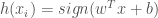
Figure 1: A hyperplane, H, that divides positive points (blue dots) and negative points (red triangles). The hyperplane’s orientation is defined by an orthogonal vector, w, which can be thought of as a vector of weights across d dimensions (in this case 3).

The Perceptron algorithm

To find the proper for data set x, Perceptron uses the following steps:

  1. Start with an initial guess of w = 0
  2. Check to see if there are any misclassified points (ie. is yi(wTxi) > 0 for all xi?)
  3. If any point is found is to be misclassified, it is added to w, creating a new hyperplane
  4. With the updated w, loop through all points again checking for misclassification and update if necessary
  5. Continue until there are no misclassfied points remaining (ie the algorithm has converged)

It can be formally proven that if the data is linearly separable, Perceptron will converge in a finite number of updates.

I should note that while this discussion of perceptron has used geometric intuition to explain the algorithm (which is how professor Weinberger teaches it in his 4780 class and how I find it easiest to understand), many people conceptualize Perceptron as a step function and w as the weights for each input to this function. While this results in exactly the same thing as the above description, if you think this may be an easier way to understand, see this link.

Problems with Perceptron

While Perceptron does not suffer from the curse of dimensionality as K-NN does, it is still highly limited in its capabilities as it will never converge on data that is not linearly separable (such as the famous XOR problem demonstrated by Minsky and Papert). Luckily for us many more techniques have been developed to handle such data sets since the late 60’s when their book was written! Stay tuned for future posts for more machine learning topics.

References

1: “New Navy Device Learns By Doing” the New York Times, 7/8/1958 (These seem like fairly grandiose claims for such a small column, just saying)

Intro to Machine Learning: Classification using K-NN

Rohini and I are taking Kilian Weinberger’s fantastic machine learning class here at Cornell this semester and I thought I’d use a couple blog posts to share what we’ve been learning. I hope these posts can serve as a look into the topics covered in this class and what is meant by the term “machine learning”, which is a hot topic these days. In these posts I’ll provide overviews of the topics we’re learning and some example code. There is way more material in this class than could every be covered on this blog and if you’re interested in learning more on the subject I’d suggest checking out the course web page where all lecture video links and lecture notes (where the content in this post is derived from) are free an open to the public.

In this post we’ll start with a very simple algorithm that you’ve probably heard of, the K-Nearest Neighbors (K-NN) algorithm. We’ll look at how K-NN is performed, why it works and the theoretical limits of its performance. We’ll then examine cases where K-NN performs poorly and learn why. The concepts in this simple example will lay the foundation for the more sophisticated Machine Learning techniques that will be discussed in future posts.

The Problem: Binary Classification

Say you have a set of data where each point has a number of features (attributes that define the point, such as an x-y coordinate) and a label such as red/blue or 1/-1. If we were given a new point and told it’s features but not it’s label, can we predict its label based on information from the data we have? We’ll call our original data set the training set, and the new point a test input.

Points_demo

Figure 1: Can we predict the classification for the new point (star) based on it’s features (x,y coordinates) and those of the training data?


The K-NN algorithm

The K-NN algorithm is based on a simple idea, that points close to each other in the feature space are likely to have similar labels. This allows us to create a classification rule:

For a test input x, assign the most common label among its k most similar training inputs

Here we are defining similarity in terms of distance within the feature space. To put the above definition formally for a new point x, the classification rule for label y of the new point, h(x) is:

h(x) = mode({y'' : (x'', y'') \in S_x})

where:

Sx is the set of k nearest neighbors of x:

S_x \subseteq D \quad s.t \enspace |S_x| =k

and \forall (x',y') \in D,S_x,

dist(x,x') \geq \underset{dist(x,x'') \in S_x}{max}(x'',y'')

KNN_k5

Figure 2: If k=5, the new point is classified as +1 because it has three +1 neighbors and two -1 neighbors.

The choice of k here is important one, for noisy data with a smooth boundary between classes, a larger k will usually be preferable. Choosing k is difficult to do a priori, and should be done by finding k that minimizes the error in a validation set and testing it over a separate testing data set to check for over fitting.

Defining a distance metric

The concept of proximity is critical to K-NN, we define a set of nearest neighbors as the k closest points to our test point in the feature space. But how do we define closeness? When we think of distances in everyday life we usually think of Euclidean distance:

dist(x,z) = \sqrt{\sum_{r=1}^{d} (x_r-z_r)^2 }

However, other distance metrics may be useful. In fact, the Euclidean distance is just one form of the more general Minkowski distance:

dist(x,z) =(\sum_{r=1}^{d} (x_r-z_r)^p)^{1/p}

Aside from the euclidean distance (p=2), other common forms of the Minkowski distance include the taxicab norm (p=1) or the infinity norm (p=infinity).

Another possible distance metric is the Mahalanobis distance, which accounts for correlation between points. For a detailed look into the use of Mahalanobis and Euclidean distance see Billy’s excellent post from earlier this year.

But how good of a classifier is K-NN?

How should we evaluate the performance of a machine learning algorithm? We can calculate the error rate of our predictions over a testing set, but this alone does not tell the full story as it neglects the properties of the testing set itself. It is therefore useful to set theoretical lower and upper bounds for error of a potential model.

The upper bound on error constitutes a classifier that our constructed model should always beat. A useful upper bound is the best constant predictor, which will always predict the most common label in the training set for any new point. If you construct a model that is able to classify points correctly 55% of the time, but 60% of the points in your data set have a certain label, you’re model is pretty useless.

Establishing the upper bound on error is pretty straight forward, but how do we specify a lower bound? What is the theoretical limit to the performance of a classification algorithm? To answer this question, lets assume we knew the probability of label y of data set x, P(y|x). We can then define the Bayes Optimal Classifier, hopt(x) as:

h_{opt}(x) = y*=\underset{y}{argmax}{P(y|x)}

We the error rate of  hopt(x)  is then defined as:

\epsilon_{BayesOpt} = 1-P(h_{opt}|y) = 1-P(y^*|x)

This error is the theoretical limit of our performance. If we new precisely the probability that a point had features x, this is the best we could do to predict its label. So how does the K-NN algorithm stack up? Cover and Hart (1967) famously proved that the error rate of a 1-NN classifier is no more than twice there error of the Bayes optimal classifier (See course notes for the full proof). Not bad!

The Curse of Dimensionality

The K-NN algorithm rests on the assumption that similar points have similar labels. As we increase the dimensionality of our feature space however, finding “similar” points becomes increasingly difficult. As we increase the number of features we are comparing, all points in our data set become more distant from each other.

As an example, lets take a look at the “similarity” between fellow Reed group member Rohini and I based on a set of features I’ve chosen at random:

Rohini v Dave

If we look at only three dimensions of features, Rohini and I are quite similar (in fact identical in terms of occupation, favorite class and current location). As we increase the number of features however, our similarity decreases precipitously. The more features we examine, the more unique each of us gets.  If we were to randomly sample these features of 100 people on campus, the similarity between Rohini and I in this feature set would likely not stand out from the sample. This is the curse of dimensionality, as the the number of features become large, the distance between all points increases to a point where it is impossible to determine “similarity” between points. If  we are unable to find neighbors that are “similar” to a test point, how can we assume any other point can be used to predict its label?

For high dimensional data sets, techniques such as PCA may make K-NN feasible if the data has a lower dimensional structure. If this isn’t effective, we must seek other strategies for classification. While the curse of dimensionality dictates that all points in a large dimensional space are distant from each other, this concept does not hold for the distance between points and hyperplanes. The Perceptron Algorithm, which I’ll cover in the next post, exploits this idea to create linear classifiers that are effective on high dimensional data.


Google Dataset Search (beta): Revolutionize your Data Searches and Database Exposure

Google just released the (beta) version of a dataset search a couple days ago (Dataset Search Link), allowing users to effectively and efficiently search publicly available databases. With the use of Google-fu (a quick  graphic guide) or even regular Google skills, discovering data sets that might be buried in a web page are more readily discoverable.

Conversely, better standardization of your datasets allows for an increased likelihood that it will reach broader audiences in the near future. Google has set forth guidelines that you should consider following to ensure exposure.

Example Dataset Search

Say we’re interested in finding potential databases that might contain information on crop allocation in California without being aware of any well-known sources; if you already have a database to access the data you need, just head there first. With a simple search, we can identify any potentially available dataset and explore its contents. example_search_labeledIn this specific example, we were able to discover that the National Agricultural Statistics Service has a raster dataset called the Cropland Data Layer that shows annual crop-specific land cover for the entire continental United States that was created using moderate-resolution satellite imagery and validated/corrected with agriculture ground truth. (Notably, CropScape has its own web-based GIS viewer, shown below)crop_example.PNG

Database Guidelines Overview

As previously mentioned, Google has established guidelines that will increase the likelihood that your dataset may be found via this new tool. Notably, they recommend that your site should be marked up using JSON-LD (Microdata and RDFa are also supported). For help, use the standardized Schema.org to ensure you have the proper setup for your website’s markup (i.e. the HTML code describing webpage that can be “read” by Google and web browsers). Dataset-specific vocabulary is shown here and is also shown on as examples on the Google Datasets Guide.

Google has a created Structured Data Markup Helper to help generate the necessary HTML code. They note that you can test your data set using the following tool either using the code snippet for your webpage or by fetching the URL itself (link to tool). If you need additional help, Google’s forums are a valuable resource.

Establishing an Effective Data Backup Strategy for Your Workstation

When determining your data management strategy for your workflow, considering a range of backup options for your data beyond just a single copy on your workstation or your external hard drive is paramount. Creating a seamless workspace that will easily transition between workstations and while maintaining durability and availability is easily achievable once you know what resources might be available and a general guideline.

General considerations for how you will be managing and sharing data is crucial, especially for collaborative projects when files must often be accessible in real time.

Considering how long you might need to retain data and how often you might need to access it will drastically change your approach to your storage strategy.

3-2-1 Data Backup Rule

If you walk away form this with nothing else, remember the 3-2-1 rule. The key to ensuring durability of your data—preventing loss due to hardware or software malfunction, fire, viruses, and institutional changes or uproars—is following the 3-2-1 Rule. Maintaining three or more copies on two or more different mediums (i.e. cloud and HDD) with at least one off-site copy.

3-2-1-Backup-Rule-1024x505Source: https://cactus-it.co.uk/the-3-2-1-backup-rule/

An example of this would be to have a primary copy of your data on your desktop that is backed up continuously via Dropbox and nightly via an external hard drive. There are three copies of your data between your local workstation, external hard drive (HD), and Dropbox. By having your media saved on hard drive disks (HDDs) on your workstation and external HD in addition to ‘the cloud’ (Dropbox), you have accomplished spreading your data across exactly two different mediums. Lastly, since cloud storage is located on external servers connected via the internet, you have successfully maintained at least one off-site copy. Additionally, with a second external HD, you could create weekly/monthly/yearly backups and store this HD offsite.

Version Control Versus Data Backup

Maintaining a robust version control protocol does not ensure your data will be properly backed up and vice versa. Notably, you should not be relying on services such as GitHub to back up your data, only your code (and possibly very small datasets, i.e. <50 MB). However, you should still maintain an effective strategy for version control.

  • Code Version Control
  • Large File Version Control
    • GitHub is not the place to be storing and sharing large datasets, only the code to produce large datasets
    • Git Large File Storage (LFS) can be used for a Git-based version-control on large files

Data Storage: Compression

Compressing data reduces the amount of storage required (thereby reducing cost), but ensuring the data’s integrity is an extremely complex topic that is continuously changing. While standard compression techniques (e.g. .ZIP and HDF5) are generally effective at compression without issues, accessing such files requires additional steps before having the data in a usable format (i.e. decompressing the files is required).  It is common practice (and often a common courtesy) to compress files prior to sharing them, especially when emailed.

7-Zip is a great open-source tool for standard compression file types (.ZIP, .RAR) and has its own compression file type. Additionally, a couple of guides looking into using HDF5/zlib for NetCFD files are located here and here.

Creating Your Storage Strategy

To comply with the 3-2-1 strategy, you must actively choose where you wish to back up your files. In addition to pushing your code to GitHub, choosing how to best push your files to be backed up is necessary. However, you must consider any requirements you might have for your data handling:

My personal strategy costs approximately $120 per year. For my workstation on campus, I primarily utilize DropBox with a now-outdated version control history plugin that allows for me to access files one year after deletion. Additionally, I instantaneously sync these files to GoogleDrive (guide to syncing). Beyond these cloud services, I utilize an external HDD that backs up select directories nightly (refer below to my script that works with Windows 7).

It should be noted that Cornell could discontinue its contracts with Google so that unlimited storage on Google Drive is no longer available. Additionally, it is likely that Cornell students will lose access to Google Drive and Cornell Box upon graduation, rendering these options impractical for long-term or permanent storage.

  • Minimal Cost (Cornell Students)
    • Cornell Box
    • Google Drive
    • Local Storage
    • TheCube
  • Accessibility and Sharing
    • DropBox
    • Google Drive
    • Cornell Box (for sharing within Cornell, horrid for external sharing)
  • Minimal Local Computer Storage Availability
    Access Via Web Interface (Cloud Storage) or File Explorer

    • DropBox
    • Google Drive (using Google Stream)
    • Cornell Box
    • TheCube
    • External HDD
  • Reliable (accessibility through time)
    • Local Storage (especially an external HDD if you will be relocating)
    • Dropbox
    • TheCube
  • Always Locally Accessible
    • Local Storage (notably where you will be utilizing the data, e.g. keep data on TheCube if you plan to utilize it there)
    • DropBox (with all files saved locally)
    • Cornell Box (with all files saved locally)
  • Large Capacity (~2 TB total)
    • Use Cornell Box or Google Drive
  • Extremely Large Capacity (or unlimited file size)

Storage Option Details and Tradeoffs

Working with large datasets can be challenging to do between workstations, changing the problem from simply incorporating the files directly within your workflow to interacting with the files from afar (e.g. keeping and utilizing files on TheCube).

But on a personal computer level, the most significant differentiator between storage types is whether you can (almost) instantaneously update and access files across computers (cloud-based storage with desktop file access) or if manual/automated backups occur. I personally like to have a majority of my files easily accessible, so I utilize Dropbox and Google Drive to constantly update between computers. I also back up all of my files from my workstation to an external hard drive just to maintain an extra  layer of data protection in case something goes awry.

  • Requirements for Data Storage
  • Local Storage: The Tried and True
    • Internal HDD
      • Installed on your desktop or laptop
      • Can most readily access data for constant use, making interactions with files the fastest
      • Likely the most at-risk version due to potential exposure to viruses in addition to nearly-constant uptime (and bumps for laptops)
      • Note that Solid State Drives (SSDs) do not have the same lifespan for the number of read/write as an HDD, leading to slowdowns or even failures if improperly managed. However, newer SSDs are less prone to these issues due to a combination of firmware and hardware advances.
      • A separate data drive (a secondary HDD that stores data and not the primary operating system) is useful for expanding easily-accessible space. However, it is not nearly as isolated as data contained within a user’s account on a computer and must be properly configured to ensure privacy of files
    • External Hard Drive Disk (HDD)
      • One-time cost ($50-200), depending on portability/size/speed
      • Can allow for off-line version of data to be stored, avoiding newly introduced viruses from preventing access or corrupting older versions (e.g. ransomware)—requires isolation from your workflow
      • May back up data instantaneously or as often as desired: general practice is to back up nightly or weekly
      • Software provided with external hard drives is generally less effective than self-generated scripts (e.g. Robocopy in Windows)
      • Unless properly encrypted, can be easily accessed by anyone with physical access
      • May be used without internet access, only requiring physical access
      • High quality (and priced) HDDs generally increase capacity and/or write/read speeds
    • Alternative Media Storage
      • Flash Thumb Drive
        • Don’t use these for data storage, only temporary transfer of files (e.g. for a presentation)
        • Likely to be lost
        • Likely to malfunction/break
      • Outdated Methods
        • DVD/Blu-Ray
        • Floppy Disks
        • Magnetic Tapes
      • M-Discs
        • Required a Blu-Ray or DVD reader/writer
        • Supposedly lasts multiple lifetimes
        • 375 GB for $67.50
  •  Dropbox
    • My experience is that Dropbox is the easiest cloud-storage solution to use
    • Free Version includes 2 GB of space without bells and whistles
    • 1 TB storage for $99.00/year
    • Maximum file size of 20 GB
    • Effective (and standard) for filesharing
    • 30-day version history (extended version history for one year can be purchased for an additional $39.00/year)
    • Professional, larger plans with additional features (e.g. collaborative document management) also available
    • Can easily create collaborative folders, but storage counts against all individuals added (an issue if individuals are sharing large datasets)
    • Can interface with both a web interface and across as operating system desktops
    • Fast upload/download speeds
    • Previous version control can allow access to previous versions if ransomware becomes an issue
    • Supports two-factor authentication
    • Requires internet access for online storage/backup, but has offline access
  • Google Drive
    • My experience is that Google Drive is relatively straight forward
    • Unlimited data/email storage for Cornell students, staff, and faculty
    • Costs $9.99/mo for 1 TB
    • Maximum file size of 5 GB
    • Easy access to G Suite, which allows for real-time collaboration on browser-based documents
    • Likely to lose access to storage capabilities upon graduation
    • Google Drive is migrating over to Google Stream which stores less commonly used files online as opposed to on your hard drive
    • Google File Stream (used to sync files with desktop) requires a constant internet connection except for recently-used files
    • Previous version control can allow access to previous versions if ransomware becomes an issue
    • Supports two-factor authentication
    • Requires internet access for online storage/backup
  • Cornell Box
    • My experiences are that Cornell Box is not easy to use relative to other options
    • Unlimited storage space, 15 GB file-size limit
    • Free for Cornell students, staff, and faculty, but alumni lose access once graduating
    • Can only be used for university-related activities (e.g. classwork, research)
    • Sharable links for internal Cornell users; however, it is very intrusive to access files for external users (requires making an account)
    • Version history retains the 100 most recent versions for each file
    • Can connect with Google Docs
    • Previous version control can allow access to previous versions if ransomware becomes an issue
    • Supports two-factor authentication
    • Requires internet access for online storage/backup, but has offline access
  • TheCube

Long-Term (5+ Years) Data Storage

It should be noted that most local media types degrade through time. Utilizing the 3-2-1 strategy is most important for long-term storage (with an emphasis on multiple media types and off-site storage). Notably, even if stored offline and never used, external HDDs, CDs, and Blu-Ray disks can only be expected to last at most around five years. Other strategies, such as magnetic tapes (10 years) or floppy disks (10-20 year), may last longer, there is no truly permanent storage strategy (source of lifespans).

M-Discs are a write-once (i.e. read only, cannot be modified) storage strategy that is projected to last many lifetimes and up to 1,000 years. If you’re able to dust off an old Blu-Ray disk reader/writer, M-Discs are likely the best long-term data strategy that is likely to survive the test of time—making two copies stored in two locations is definitely worthwhile. However, the biggest drawback is that M-Discs are relatively difficult to access compared to plugging in an external HD.

Because of the range of lifespans and how cheap storage has become, I would recommend maintaining your old (and likely relatively small) data archives within your regular storage strategy which is likely to migrate between services through time.

For larger datasets that you are required to retain and would like to easily access, I would maintain them on at least two offline external hard drive stored in separate locations (e.g. at home and your office) while occasionally (i.e. every six months) checking the health of the hard drives in perpetuity and replacing them as required.

Relying only on cloud storage for long-term storage is not recommended due to the possibility of companies closing their doors or simply deactivating your account. However, they can be used as an additional layer of protection in addition to having physical copies (i.e. external HD, M-Discs).

Windows 7 Robocopy Code

The script I use for backing up specific directories from my workstation (Windows 7) to an external HD is shown below. To set up my hard drive, I first formatted it to a format compatible with multiple operating systems using this guide. Note that your maximum file size and operating system requirements require different formats. Following this, I used the following guide to implement a nightly backup of all of my data while keeping a log on my C: drive. Note that I have only new files and versions of files copied over, ensuring that the back up does not take ages.

@echo off
robocopy C:\Users\pqs4\Desktop F:\Backups\Desktop /E /XA:H /W:0 /R:3 /REG > C:\externalbackup.log
robocopy E:\Dropbox F:\Backups\Dropbox /E /XA:SH /W:0 /R:3 /REG /XJ >> C:\externalbackup.log
robocopy C:\Users\pqs4\Downloads F:\Backups\Downloads /E /XA:SH /W:0 /R:3 /REG /XJ >> C:\externalbackup.log
robocopy C:\Users\pqs4\Documents F:\Backups\Documents /E /XA:SH /W:0 /R:3 /REG /XJ >> C:\externalbackup.log
robocopy C:\Users\pqs4 F:\Backups\UserProfile /E /XA:SH /W:0 /R:3 /REG /XJ >> C:\externalbackup.log
robocopy E:\Program Files\Zotero F:\Backups\Zotero /E /XA:SH /W:0 /R:3 /REG /XJ >> C:\externalbackup.log

Implementation of the Moving Average Filter Using Convolution

What is convolution?

Convolution is an operation that is performed between two signals to produce a third signal that represents how one input signal modifies the other. The convolution h(t) of two signals, f(t) and g(t), is defined as:

capture.png

or more concisely,

Capture1

where * represents the convolution operator. The former equation can also be written discretely as:

capture21.png

where f(t) and g(t) are no longer continuous signals, but rather discrete sequences of numbers (vectors).

The steps to perform a convolution can be summarized as follows:

Step 1: Replace the variable t in f(t) and g(t) with a dummy variable u to obtain f(u) and g(u).

Step 2: Flip the second signal to obtain g(-u).

Step 3: Shift the flipped signal by t to get g(t-u), so that the signal can slide along the u axis.

Step 4: Start t at -∞ and wherever the two functions intersect, find the integral of their product.

Step 5: Continue shifting and integrating until second signal has completely passed over the first signal. The result, h(t), is the convolution of f(t) and g(t).

The animation below illustrates the convolution of a boxcar signal with itself, resulting in a triangle function.

Convolution_of_box_signal_with_itself2

Convolution of Two Boxcar Functions1

Convolution is used extensively in signal processing to determine the output of a system as a response to a set of inputs, but it has applications in many fields.  For example, in image processing, an image (essentially an array) can be convolved with a 2D kernel (a smaller array) that, depending on the kernel size and values, can be used to blur, sharpen, or detect edges in an image. Convolution is also implemented in audio processing to simulate reverberation or to produce new sounds. Other applications that utilize convolution include neural networks, optics, and probability theory2. Perhaps most relevant to the field of water resources is the use of convolution to create a moving average.

Moving Average

A moving average is a form of a convolution often used in time series analysis to smooth out noise in data by replacing a data point with the average of neighboring values in a moving window. A moving average is essentially a low-pass filter because it removes short-term fluctuations to highlight a deeper underlying trend.

The mathematical definition of a moving average is:

Capture4

where the average data point is calculated from averaging the points contained in the moving window that is defined as +/- M and centered around xi .

A moving average is commonly referred to as boxcar smoothing because it is implemented by convolving the time series signal with a box-shaped function of width 2M+1,  with an amplitude of 1/(2M+1).

Shown below is an example of how a moving average can be implemented using both the convolution function and the Astropy library in Python.

Example: Daily Minimum Temperatures in Melbourne, Australia

Figure 1 is a graph of daily minimum temperatures in Melbourne, Australia from 1981-1990. Our goal is to use a moving average to smooth out some of the noise in this graph to highlight the underlying signal.

Figure_2

Figure 1: Daily Minimum Temperatures in Melbourne

The first step is to read in the raw data, which can be downloaded here. Then, define a window size, w, that is equal to 2M+1. Choosing the width of the moving window is not trivial and very application-specific. If the window is too big, the trends in the data may be masked, while too small of a window may not show the larger underlying trend. Therefore, you must have some intuition as to what trends might lie in the data. If the data are seasonal or periodic in nature, consider choosing a window size consistent with the seasonality. Because daily minimum temperatures will have a seasonal component depending on the month of the year, the window width is set at 31 (30 days+1 to account for the center point).

"""
======================================================
Smoothing of TimeSeries Data Using Convolution
======================================================

"""
#Import libraries 

import matplotlib.pyplot as plt
import numpy as np
from pandas import Series

#Upload raw data as a pandas series

series = Series.from_csv('daily-minimum-temperatures.csv')

#Define window size
w=31

Then, a mask is created that is a vector of length w, with each element having a value of 1/w (a boxcar signal of length w and amplitude 1/w).

#Define mask and store as an array
mask=np.ones((1,w))/w
mask=mask[0,:]

The final step is to convolve the data with the boxcar signal and plot the final result, shown in Figure 2.

#Convolve the mask with the raw data
convolved_data=np.convolve(series,mask,'same')

#Change series to data frame and add convolved data as a new column
series=Series.to_frame(series)
series['convolved_data']=convolved_data

#Plot both original and smooth data
plt.ylabel('Temperature (C)')
plt.xlabel('Time')
plt.title('Daily Minimum Temperatures in Melbourne (1981-1990)')
plt.plot(series)
plt.legend(('Original','Smooth'))
plt.show()

Because I wanted the output signal to be the same length as the input signal, I used the parameter option, “same” which will add a padding of zeros around the boundaries of the data to preserve the length. The effect of this can be seen by the sharp boundaries of the smooth data. Other parameter options such as “valid” will only return points that fall inside the intersection of the two signals.

Figure_3

Figure 2: Original and Smooth Temperature Data

Once you understand the math behind the moving average, you can easily do the same convolution in a single line using the AstroPy library.

from astropy.convolution import convolve, Box1DKernel
smooth_data=convolve(series,kernel=Box1DKernel(31))

Sources:

All information not specifically cited came from class notes from Dr. Greg McLaskey’s class, CEE 6790: Times Series Data Analysis for Civil, Mechanical, and Geophysical Applications

[1] Animation authorship details here

[2]https://www.allaboutcircuits.com/technical-articles/dsp-applications-of-convolution-part-2/