Fans of this blog will know that uncertainty is often a focus for our group. When approaching uncertainty, Bayesian methods might be of interest since they explicitly provide uncertainty estimates during the modeling process.
PyMC is the best tool I have come across for Bayesian modeling in Python; this post gives a super brief introduction to this toolkit.
Introduction to PyMC
PyMC, described in their own words: “… is a probabilistic programming library for Python that allows users to build Bayesian models with a simple Python API and fit them using Markov chain Monte Carlo (MCMC) methods.”
In my opinion, the best part of PyMC is the flexibility and breadth of model design features. The space of different model configurations is massive. It allows you to make models ranging from simple linear regressions (shown here), to more complex hierarchical models, copulas, gaussian processes, and more.
Regardless of your model formulation, PyMC let’s you generate posterior estimates of model parameter distributions. These parameter distributions reflect the uncertainty in the model, and can propagate uncertainty into your final predictions.
The posterior estimates of model parameters are generated using Markov chain Monte Carlo (MCMC) methods. A detailed overview of MCMC is outside the scope of this post (maybe in a later post…).
In the simplest terms, MCMC is a method for estimating posterior parameter distributions for a Bayesian model. It generates a sequence of samples from the parameter space (which can be huge and complex), where the probability of each sample is proportional to its likelihood given the observed data. By collecting enough samples, MCMC generates an approximation of the posterior distribution, providing insights into the probable values of the model parameters along with their uncertainties. This is key when the models are very complex and the posterior cannot be directly defined.
When writing drafting this post, I wanted to include a demonstration which is (a) simple enough to cover in a brief post, and (b) relatively easy for others to replicate. I settled on the simple linear regression model described below, since this was able to be done using readily retrievable CAMELS data.
The example attempts to predict mean streamflow as a linear function of basin catchment area (both in log space). As you’ll see, it’s not the worst model, but its far from a good model; there is a lot of uncertainty!
CAMELS Data
For a description of the CAMELS dataset, see Addor, Newman, Mizukami and Clark (2017).
I pulled all of the national CAMELS data using the pygeohydro package from HyRiver which I have previously recommended on this blog. This is a convenient single-line code to get all the data:
import pygeohydro as gh

### Load camels data
camels_basins, camels_qobs = gh.get_camels()
The camels_basins variable is a dataframe with the different catchment attributes, and the camels_qobs is a xarray.Dataset. In this case we will only be using the camels_basins data.
The CAMELS data spans the continental US, but I want to focus on a specific region (since hydrologic patterns will be regional). Before going further, I filter the data to keep only sites in the Northeaster US:
# filter by mean long lat of geometry: NE US
camels_basins['mean_long'] = camels_basins.geometry.centroid.x
camels_basins['mean_lat'] = camels_basins.geometry.centroid.y
camels_basins = camels_basins[(camels_basins['mean_long'] > -80) & (camels_basins['mean_long'] < -70)]
camels_basins = camels_basins[(camels_basins['mean_lat'] > 35) & (camels_basins['mean_lat'] < 45)]
I also convert the mean flow data (q_mean) units from mm/day to cubic meters per day:
# convert q_mean from mm/day to m3/s
camels_basins['q_mean_cms'] = camels_basins['q_mean'] * (1e-3) *(camels_basins['area_gages2']*1000**2) * (1/(60*60*24))
And this is all the data we need for this crude model!
Bayesian linear model
The simple linear regression model (hello my old friend):
Normally you might assume that there is a single, best value corresponding to each of the model parameters (alpha and beta). This is considered a Frequentist perspective and is a common approach. In these cases, the best parameters can be estimated by minimizing the errors corresponding to a particular set of parameters (see least squares, for example.
However, we could take a different approach and assume that the parameters (intercept and slope) are random variables themselves, and have some corresponding distribution. This would constitute a Bayesian perspective.
Keeping with simplicity in this example, I will assume that the intercept and slope each come from a normal distribution with a mean and variance such that:
When it comes time to make inferences or predictions using our model, we can create a large number of predictions by sampling different parameter values from these distributions. Consequently, we will end up with a distribution of uncertain predictions.
NOTE: The MCMC sampler used by PyMC is written in C and will be SIGNIFICANTLY faster if you provide have access to GCC compiler and specify the it’s directory using the the following:
import pymc as pm

import os
os.environ["THEANO_FLAGS"] = "gcc__cxxflags=-C:\mingw-w64\mingw64\bin"
You will get a warning if you don’t have this properly set up.
Now, onto the demo!
I start by retrieving our X and Y data from the CAMELS dataset we created above:
# Pull out X and Y of interest
x_ftr= 'area_gages2'
y_ftr = 'q_mean_cms'
xs = camels_basins[x_ftr]
ys = camels_basins[y_ftr]

# Take log-transform
xs = np.log(xs)
ys = np.log(ys)
At a glance, we see there is a reasonable linear relationship when working in the log space:
Two of the key features when building a model are:
The random variable distribution constructions
The deterministic model formulation
There are lots of different distributions available, and each one simply takes a name and set of parameter values as inputs. For example, the normal distribution defining our intercept parameter is:
The value of the parameter priors that you specify when construction the model may have a big impact depending on the complexity of your model. For simple models you may get away with having uninformative priors (e.g., setting mu=0), however if you have some initial guesses then that can help with getting reliable convergence.
In this case, I used a simple least squares estimate of the linear regression as the parameter priors:
Once we have our random variables defined, then we will need to formulate the deterministic element of our model prediction. This is the functional relationship between the input, parameters, and output. For our linear regression model, this is simply:
y_mu = alpha + beta * xs
In the case of our Bayesian regression, this can be thought of as the mean of the regression outputs. The final estimates are going to be distributed around the y_mu with the uncertainty resulting from the combinations of our different random variables.
Putting it all together now:
### PyMC linear model
with pm.Model() as model:

    # Priors
    alpha = pm.Normal('alpha', mu=intercept_prior, sigma=10)
    beta = pm.Normal('beta', mu=slope_prior, sigma=10)
    sigma = pm.HalfNormal('sigma', sigma=1)

    # mean/expected value of the model
    mu = alpha + beta * xs

    # likelihood
    y = pm.Normal('y', mu=mu, sigma=sigma, observed=ys)

    # sample from the posterior
    trace = pm.sample(2000, cores=6)
With our model constructed, we can use the pm.sample() function to begin the MCMC sampling process and estimate the posterior distribution of model parameters. Note that this process can be very computationally intensive for complex models! (Definitely make sure you have the GCC set up correctly if you plan on needing to sample complex models.)
Using the sampled parameter values, we can create posterior estimates of the predictions (log mean flow) using the posterior parameter distributions:
Let’s go ahead and plot the range of the posterior distribution, to visualize the uncertainty in the model estimates:
### Plot the posterior predictive interval
fig, ax = plt.subplots(ncols=2, figsize=(8,4))

# log space
az.plot_hdi(xs, ppc['posterior_predictive']['y'],
            color='cornflowerblue', ax=ax[0], hdi_prob=0.9)
ax[0].scatter(xs, ys, alpha=0.6, s=20, color='k')
ax[0].set_xlabel('Log ' + x_ftr)
ax[0].set_ylabel('Log Mean Flow (m3/s)')

# original dim space
az.plot_hdi(np.exp(xs), np.exp(ppc['posterior_predictive']['y']),
            color='cornflowerblue', ax=ax[1], hdi_prob=0.9)
ax[1].scatter(np.exp(xs), np.exp(ys), alpha=0.6, s=20, color='k')
ax[1].set_xlabel(x_ftr)
ax[1].set_ylabel('Mean Flow (m3/s)')
plt.suptitle('90% Posterior Prediction Interval', fontsize=14)
plt.show()
And there we have it! The figure on the left shows the data and posterior prediction range in log-space, while the figure on the right is in non-log space.
As mentioned earlier, it’s not the best model (wayyy to much uncertainty in the large-basin mean flow estimates), but at least we have the benefit of knowing the uncertainty distribution since we took the Bayesian approach!
That’s all for now; this post was really meant to bring PyMC to your attention. Maybe you have a use case or will be more likely to consider Bayesian approaches in the future.
If you have other Bayesian/probabilistic programming tools that you like, please do comment below. PyMC is one (good) option, but I’m sure other people have their own favorites for different reasons.
Addor, N., Newman, A. J., Mizukami, N. and Clark, M. P. The CAMELS data set: catchment attributes and meteorology for large-sample studies, Hydrol. Earth Syst. Sci., 21, 5293–5313, doi:10.5194/hess-21-5293-2017, 2017.
I recently completed a course Final Project in which I attempted to implement a Hidden Markov Model (HMM) parameterized using the Markov Chain Monte Carlo method. In this post, I will briefly introduce HMM models as well as the MCMC method. I will then walk you through an exercise implementing a HMM in the Julia programming language and share some preliminary results from my exploration in combining both these methods. All the code found in this exercise can be located in this GitHub repository.
Note: The exercise in this post will require some familiarity with Julia. For a quick introduction to this relatively recent newcomer to the programming languages scene, please refer to Peter Storm’s blog post here.
Hidden Markov Models
A Hidden Markov Model (HMM) is a statistical tool used to model different types of time series data ranging from signal processing, hydrology, financial statistics, speech recognition, and econometrics (Rabiner, 1990; Rydén, 2008), where the underlying process is assumed to be Markovian. Specifically, it has been found to be effectively at modeling systems with long-term persistence, where past events have effects on current and future events at a multi-year scale (Akintug and Rasmussen, 2005; Bracken et al., 2014). Recent studies have also found that it is possible to use HMMs to model the dynamics of streamflow, where the HMM state space represents the different hydrological conditions (e.g. dry vs. wet) and the observation space represents the streamflow data (Hadjimichael et al., 2020; 2020a). These synthetic streamflows are computationally generated with the aid of packages such as hmmlearn in Python and HMMBase in Julia. An example implementation of hmmlearn can be found in Julie Quinn’s blog post here. She also wrote the prequel to the implementation post, where she dives into the background of HMMs and applying Expectation-Maximization (EM) to parameterize the model.
Markov Chain Monte Carlo
The EM approach of parameterizing HMMs reflects a frequentist approach that assumes the existence of one “true” value for each HMM parameter. In this exercise, I will instead use a Bayesian approach via the Markov Chain Monte Carlo method to generate and randomly sample potential parameter (model prior) values from a Markov chain, which are statistical models that approximate Markovian time series. In these time series, the probability of being in any given state st at current time t is dependent only on states prior to st. Using the MCMC approach, a Markov Chain is constructed for each HMM parameter such that its stationary distribution (distribution of the parameters at equilibrium) is the distribution of its associated model posterior (the likelihood of a model structure after, or a posteriori, obtaining system observed data). The model priors (assumed model structure prior to having any knowledge about the system) are randomly sampled from their respective chains — hence the term “Monte Carlo”. These samples are then used to estimate the statistical properties of the distribution of each parameter.
Overall, MCMC is a powerful method to estimate the statistical properties of high-dimensional problems with many parameters. Nonetheless, it is beholden to its own set of limitations that include high computational expense and the inability to guarantee convergence. Figure 1 below summarize some of the benefits and drawbacks of using MCMC parameterization:
Figure 1: The pros and cons of using MCMC parameterization.
Setting up the parameters
In this exercise, I will be using the HMM to approximate the statistical properties of streamflow data found in the annualQ.csv file previously used also by Rohini in her post on creating HMMs to generate synthetic streamflow seriesand by the MSD UC Ebook HMM training Jupyter Notebook. This streamflow time series originated from a USGS outlet gauge in the Upper Colorado River Basin. It records 105 years’ worth of streamflow from 1909 and 2013 (inclusive). It was previously found that it was best described using two states (wet and dry; Bracken et al, 2014). In this exercise, I also assume that this time series is best approximated by a first-order HMM where the state at current time t (st) is only affected by the state at the timestep immediately prior to it (st-1).
In this exercise, I will be using MCMC to parameterize the following HMM parameters:
Parameter
Description
The initial state distribution a for wet (1) and dry (2) states
The transition matrix A from a wet (1) to a dry (2) state
The probability distributions for the vector of observations x for a given state where Wet: 1 and Dry: 2
Table 1: Summary of all HMM parameters to be adjusted using the MCMC approach.
From Table 1 above:
P(ai) is the initial state probability for state i
P(Aij) is the transition probability from state i to state j
μiand σi are the mean and standard deviation for the vector of streamflow observations x for a given state i
Now that the dataset and model parameters have been introduced, we will proceed with demonstrating the code required to implement the HMM model with MCMC parameterization.
Implementing the streamflow HMM with using MCMC parameterization
Before begin, I recommend downloading and installing Julia 1.8.5. Please find the Windows and Mac 64-bit installer here. Once Julia is set up, we can download and install all required packages. In Julia, this can be done as follows:
# make sure all required packages are installed
import Pkg
Pkg.activate(@__DIR__);
Pkg.instantiate();
Once this is done, we can load all the required packages. In Julia, this is done using the using key word, which can be thought of as the Python import parallel. Note that I placed a semicolon after the using CSV line. This is to prevent the automatic printing of output messages that Julia automatically displays when loading packages.
# load all packages
using Random
using CSVFiles # load CSV data
using DataFrames # data storage and presentation
using Plots # plotting library
using StatsPlots # statistical plotting
using Distributions # statistical distribution interface
using Turing # probabilistic programming and MCMC
using Optim # optimization library
using StatsBase
using LaTeXStrings
using HMMBase
using DelimitedFiles
using CSV;
Now, let’s load the data and identify the number of years and number of states inherent to time streamflow time series.
# load data
# source: https://github.com/IMMM-SFA/msd_uncertainty_ebook/tree/main/notebooks/data
Q = CSV.File("annualQ.csv", header=[:Inflow]) |> DataFrame
Q = Q[2:end,:]
Q[!,:Inflow] = parse.(Float64, Q[!, :Inflow])
Q[!, :Year] = 1909:2013;
Q[!, :logQ] = log.(Q[!, :Inflow]);

# Assume first-order HMM where only the immediate prior step influences the next step
n_states = 2
logQ = Q[!,:logQ];
n_years = size(logQ)[1];
Next, we should set a random seed to ensure that our following results are consistent. This is because the package that we are using in this exercise called “Distributions” performs random sampling. Without setting the seed (shown below), the outcomes of the exercise may be wildly different each time the MCMC parameterization algorithm is run.
# Set the random seed
Random.seed!(1)
Next, we define the HMM model with MCMC sampling. The sampling is performed using methods and syntax built into the Turing.jl package. In the code below, also note lines 32 to 38. Within those lines, the observations’ states are enforced where observations with log-streamflows below the input mean are assigned to a dry state, while the opposite is implemented for log-streamflows above the wet state. This step is important to prevent mode collapse, where the HMM model cannot distinguish between the wet and dry state distributions due to the random sampling of the MCMC parameterization.
@model function HMM_mcmc(logQ, n_states, n_years)
    # Source: https://chat.openai.com/c/d81ef577-9a2f-40b2-be9d-c19bf89f9980
    # Prompt example: Please suggest how you would parameterize Hidden Markov Model with the Markov Chain Monte Carlo method
    # Uses the Turing.jl package in Julia. The input to this model will be an inflow timeseries with two hidden states.
    mean_logQ = mean(logQ)

    # Define the prior distributions for the parameters
    μ₁ ~ Normal(15.7, 0.25)   # wet state
    μ₂ ~ Normal(15.2, 0.25)   # dry state
    σ₁ ~ truncated(Normal(0.24, 0.1), 0, Inf)
    σ₂ ~ truncated(Normal(0.24, 0.1), 0, Inf)
    a11 ~ Dirichlet(ones(n_states))
    A ~ filldist(Dirichlet(ones(n_states)), n_states)
    s = tzeros(Int, n_years)   # Define the vector of hidden states

    # Define intial state probability distribution
    a = [a11[1], 1-a11[1]]   # [wet state, dry state]

    # Define the observation distributions
    B = [Normal(μ₁, σ₁), Normal(μ₂, σ₂)]

    # Sample the initial hidden state and observation variables
    s[1] ~ Categorical(a)

    # Loop over time steps and sample the hidden+observed variables
    for t in 2:n_years
        s[t] ~ Categorical(A[:,s[t-1]])
    end
    for t in 1:n_years
        logQ[t] ~ B[s[t]]

        # if the logQ is greater than the input mean, force the state to be a wet state
        if logQ[t] > mean_logQ
            s[t] ~ Categorical(A[:,1])
        # if the logQ is smaller than the input mean, force the state to be a dry state
        elseif logQ[t] < mean_logQ
            s[t] ~ Categorical(A[:,2])
        end

    end
end
We then have to run the model for at least 3,000 iterations before the sample values for each parameter converge to stable values. The code to perform this is as follows:
# run for 3000 iterations; usually enough
# run using >3 chains to double check convergence if desired
hmm_model = HMM_mcmc(logQ, n_states, n_years)
g = Gibbs(HMC(0.05, 10, :μ₁, :μ₂, :σ₁, :σ₂, :a11, :A), PG(10, :s))
chains = sample(hmm_model, g, MCMCThreads(), 3000, 1, drop_warmup=true)
To check for convergence, you can attempt to run plot(chains) to check for convergence, and corner(chains) to examine the parameters for dependencies. In this post, we will not discuss MCMC convergence in detail, but some things to look out for would be r_hat values in the output of the code shown above that are close to 1, as well as chains that are similar to each other. Refer to Table 2 and Figure 2 for some quick statistics that can be used as a baseline to determine if your model has converged.
Table 2: The mean converged values for some of the HMM parameters.
Figure 2: The mean converged values of the transition matrix components.
Now, let’s use the model to generate 1,000 samples of streamflow. First, we define the streamflow prediction function:
function predict_inflow(chain, logQ)
    μ₁ = Array(group(chain, :μ₁))
    μ₂ = Array(group(chain, :μ₂))
    σ₁ = Array(group(chain, :σ₁))
    σ₂ = Array(group(chain, :σ₂))
    a11 = Array(group(chain, "a11[1]"))
    a22 = Array(group(chain, "a11[2]"))
    A11 = Array(group(chain, "A[1,1]"))
    A12 = Array(group(chain, "A[1,2]"))
    A21 = Array(group(chain, "A[2,1]"))
    A22 = Array(group(chain, "A[2,2]"))

    n_samples = 1000

    μ1_sample = sample(μ₁, n_samples, replace=true);
    μ2_sample = sample(μ₂, n_samples, replace=true);
    σ1_sample = sample(σ₁, n_samples, replace=true);
    σ2_sample = sample(σ₂, n_samples, replace=true);
    a11_sample = sample(a11, n_samples, replace=true);
    a22_sample = sample(a22, n_samples, replace=true);
    A11_sample = sample(A11, n_samples, replace=true);
    A12_sample = sample(A12, n_samples, replace=true);
    A21_sample = sample(A21, n_samples, replace=true);
    A22_sample = sample(A22, n_samples, replace=true);

    Q_predict = zeros(length(logQ), n_samples)
    #residuals_ar = zeros(length(temp_data), n_samples)

    s_matrix = zeros(length(logQ), n_samples)
    logQ_matrix = zeros(length(logQ), n_samples)
    meanQ = mean(logQ)

    for n = 1:n_samples
        s_sample = tzeros(Int, n_years)
        Q_sample = zeros(n_years)

        μ1 = μ1_sample[n]
        μ2 = μ2_sample[n]
        σ1 = σ1_sample[n]
        σ2 = σ2_sample[n]
        a11 = a11_sample[n]
        a22 = a22_sample[n]
        A11 = A11_sample[n]
        A21 = 1 - A11_sample[n]
        A12 = 1 - A22_sample[n]
        A22 = A22_sample[n]
        #println(A)
        A = [A11 A12; A21 A22]
        A = transpose(A)
        #println(A)
        #a =  [1-a22, a22]
        a = [a11, 1-a11]
        print(a)
        B = [Normal(μ1, σ1), Normal(μ2, σ2)]

        # Sample the initial hidden state and observation variables
        s_sample[1] = rand(Categorical(a))

        # Loop over time steps and sample the hidden+observed variables
        for t in 2:n_years
            s_sample[t] = rand(Categorical(A[s_sample[t-1], :]))
        end
        for t in 1:n_years
            Q_sample[t] = rand(B[s_sample[t]])
            if Q_sample[t] < meanQ
                s_sample[t] = 1
            elseif Q_sample[t] > meanQ
                s_sample[t] = 2
            end
        end

        s_matrix[:, n] = s_sample
        Q_predict[:, n] = Q_sample

    end

    return s_matrix, Q_predict

end
From this function, we obtain the state and log-inflow matrix with dimensions 105 × 1000 each.
We randomly select a timeseries out of the 1,000 timeseries output by the prediction function and plot the wet and dry states identified:
# create the dry and wet masks
q = Q[!,:Inflow]
y = Q[!,:Year]

# select a random sample timeseries to plot
idx = 7
Q_wet_mcmc = q[s_matrix[:,idx] .== 1]
Q_dry_mcmc = q[s_matrix[:,idx] .== 2]

y_wet_mcmc = y[s_matrix[:,idx] .== 1]
y_dry_mcmc = y[s_matrix[:,idx] .== 2];

# plot the figure
plot(y, Q.Inflow, c=:grey, label="Inflow", xlabel="Year", ylabel="Annual inflow (cubic ft/yr)")
scatter!(y_dry_mcmc, Q_dry_mcmc, c=:salmon, label="Dry state (MCMC)", xlabel="Year", ylabel="Annual inflow (cubic ft/yr)")
scatter!(y_wet_mcmc, Q_wet_mcmc, c=:lightblue, label="Wet state (MCMC)", xlabel="Year", ylabel="Annual inflow (cubic ft/yr)")
The output figure should look similar to this:
Figure 2: Wet (pink) and dry (blue) states identified within the streamflow timeseries.
From this figure, we can see that the HMM can identify streamflow extreme as wet and dry states (albeit with some inconsistencies) where historically high streamflows are identified as a “wet state” and low streamflows are correspondingly identified as “dry”.
To make sure that the model can distinguish the observation distributions for wet and dry states, we plot their probability distribution functions. Before we plot anything, though, let’s define a function that will help us plot the distributions themselves. For this function, we first need to load the LinearAlgebra package.
# load the LinearAlgebra package
using LinearAlgebra

# function to plot the distribution of the wet and dry states
function plot_dist(Q, μ, σ, A)
    evals, evecs = eigen(A).values, eigen(A).vectors
    one_eval = argmin(abs.(evals.-1))
    π = evecs[:, one_eval] / sum(evecs[:, one_eval])

    x_0 = LinRange(μ[1] - 4*σ[1], μ[1] + 4*σ[1], 10000)
    norm0 = Normal(μ[1], σ[1])
    fx_0 = π[1].*pdf.(norm0, x_0)

    x_1 = LinRange(μ[2] - 4*σ[2], μ[2] + 4*σ[2], 10000)
    norm1 = Normal(μ[2], σ[2])
    fx_1 = π[2].*pdf.(norm1, x_1)

    x = LinRange(μ[1] - 4*σ[1], μ[2] + 4*σ[2], 10000)
    fx = π[1].*pdf.(norm0, x) .+ π[2].*pdf.(norm1, x)

    #fig, ax = plt.subplots(1, 1, figsize=(12, 8))

    b = range(μ[1] - 4*σ[1], μ[2] + 4*σ[2], length=100)

    histogram(log.(Q), c=:lightgrey, normalize=:pdf, label="Log-Inflow")
    plot!(x_0, fx_0, c=:red, linewidth=3, label="Dry State Distr", xlabel="x", ylabel="P(x)")
    plot!(x_1, fx_1, c=:blue, linewidth=2, label="Wet State Distr")
    plot!(x, fx, c=:black, linewidth=2, label="Combined State Distr")
end
Great! Now let’s use this function to plot the distributions themselves.
# get the model parameter value means
μ₁_mean = mean(chains, :μ₁)
μ₂_mean = mean(chains, :μ₂)
σ₁_mean = mean(chains, :σ₁)
σ₂_mean = mean(chains, :σ₂)
a11_mean = mean(chains, "a11[2]")
A11_mean = mean(chains, "A[1,1]")
A12_mean = mean(chains, "A[1,2]")
A21_mean = mean(chains, "A[2,1]")
A22_mean = mean(chains, "A[2,2]")

# obtained from model above
μ = [μ₂_mean, μ₁_mean]
σ = [σ₂_mean, σ₁_mean]
A_mcmc = [A11_mean 1-A11_mean; 1-A22_mean A22_mean]

# plot the distributions
plot_dist(Q[!,:Inflow], μ, σ, A_mcmc)
This code block will output the following figure:
Figure 3: The overall (black), wet (blue) and dry (red) streamflow probability distributions.
From Figure 3, we can observe that the dry state streamflow distribution is different from that of the wet state. The HMM model correctly estimates a lower mean for the dry state, and a higher one for the dry state. Based on visual analysis, the states have similar standard deviations, but this is likely an artifact of the prior parameterization of the initial HMM model that we set up earlier. The step we took earlier to force the wet/dry state distributions given a sampled log-streamflow value also likely prevented mode collapse and enabled the identification of two distinct distributions.
Now, let’s see if our HMM can be used to generate synthetic streamflow. We do this using the following lines of code:
# plot the FDC of the sampled inflow around the historical
sampled_obs_mcmc = zeros(1000, n_years)
Q_predict_mcmc = transpose(logQ_predict)
for i in 1:1000
    sampled_obs_mcmc[i,:] = exp.(Q_predict_mcmc[i, :])
    sampled_obs_mcmc[i,:] = sort!(sampled_obs_mcmc[i, :], rev=true)
end

hist_obs = copy(Q[!,:Inflow])
hist_obs = sort!(hist_obs, rev=true)
probs = (1:n_years)/n_years

plot(probs, hist_obs, c=:grey, linewidth=2, label="Historical inflow",
    xlabel="Exceedance prob.", ylabel="Annual inflow (cubic ft/yr)")
for i in 1:1000
    if i == 1
        plot!(probs, sampled_obs_mcmc[i,:], c=:lightgreen, linewidth=2,
            label="Sampled inflow (MCMC)", xlabel="Exceedance prob.", ylabel="Annual inflow (cubic ft/yr)")
    end

    plot!(probs, sampled_obs_mcmc[i,:], c=:lightgreen, linewidth=2, legend=false,
        xlabel="Exceedance prob.", ylabel="Annual inflow (cubic ft/yr)")
end

plot!(probs, hist_obs, c=:grey, linewidth=2, legend=false,
    xlabel="Exceedance prob.", ylabel="Annual inflow (cubic ft/yr)")
Once implemented, the following figure should be output:
Figure 4: The original historical streamflow timeseries (grey) and the synthetic streamflow generated by the HMM (green).
This demonstrates that the HMM model is capable of generating synthetic streamflow that approximates the statistical properties of the historical timeseries, while expanding upon the range of uncertainty in streamflow scenarios. This has implications for applications such as exploratory modeling of different streamflow scenarios, where such approaches can be used to generate a wetter- or dryer-than-historical streamflows.
Summary
While using MCMC to parameterize a HMM is a useful method to generate synthetic streamflow, one significant drawback is the long runtime and the large number of iterations that the MCMC algorithm takes to converge (Table 3).
Table 3: MCMC parameterization and runtime.
This is likely due to the HMM sampling setup. Notice that in lines 27 and 33-27 in the HMM_mcmc function: we are essentially fitting an additional probability distribution at each st essentially turning them into tunable parameters themselves. Since there are 105 elements in the streamflow timeseries, this introduces an additional 105 parameters for the MCMC to fit distributions to. This is the likely cause for the lengthy runtime. While we will not explore alternative HMM-MCMC parameterization approaches, more efficient alternatives definitely exist, and you are highly encouraged to check it out!
Overall, we began this post with a quick introduction to HMM and MCMC sampling. We then compared the pros and cons of using the MCMC approach to parameterize a HMM. Once we understood its benefits and drawbacks, we formulated a HMM for a 105-year long timeseries of annual streamflow and examined the performance of the model by analyzing its converged parameter values, observation probability distributions, as well as its ability to detect wet/dry states in the historical time series. We also used the HMM to generate 1,000 synthetic streamflow scenarios. Finally, we diagnosed the cause for the long time to convergence of the MCMC sampling approach.
This brings us to the end of the post! I hope you now have a slightly better understanding of HMMs, how they can be parameterized using the MCMC approach, as well as issues you might run into when you implement the latter.
Happy coding!
References
Akintug, B., & Rasmussen, P. F. (2005). A Markov switching model for annual hydrologic time series. Water Resources Research, 41(9). https://doi.org/10.1029/2004wr003605
Bracken, C., Rajagopalan, B., & Zagona, E. (2014). A hidden markov model combined with climate indices for Multidecadal Streamflow Simulation. Water Resources Research, 50(10), 7836–7846. https://doi.org/10.1002/2014wr015567
Hadjimichael, A., Quinn, J., & Reed, P. (2020). Advancing diagnostic model evaluation to better understand water shortage mechanisms in institutionally complex river basins. Water Resources Research, 56(10), e2020WR028079.
Hadjimichael, A., Quinn, J., Wilson, E., Reed, P., Basdekas, L., Yates, D., & Garrison, M. (2020a). Defining robustness, vulnerabilities, and consequential scenarios for diverse stakeholder interests in institutionally complex river basins. Earth’s Future, 8(7), e2020EF001503.
Reed, P.M., Hadjimichael, A., Malek, K., Karimi, T., Vernon, C.R., Srikrishnan, V., Gupta, R.S., Gold, D.F., Lee, B., Keller, K., Thurber, T.B, & Rice, J.S. (2022). Addressing Uncertainty in Multisector Dynamics Research [Book]. Zenodo. https://doi.org/10.5281/zenodo.6110623
Rydén, T. (2008). Em versus markov chain Monte Carlo for estimation of Hidden Markov models: A computational perspective. Bayesian Analysis, 3(4). https://doi.org/10.1214/08-ba326
Turek, D., de Valpine, P. and Paciorek, C.J. (2016) Efficient Markov Chain Monte Carlo Sampling for Hierarchical Hidden Markov Models, arXiv.org. Available at: https://arxiv.org/abs/1601.02698.
In this post, I will cover the very basics of Gaussian Processes following the presentations in Murphy (2012) and Rasmussen and Williams (2006) — though hopefully easier to digest. I will approach the explanation in two ways: (1) derived from Bayesian Ordinary Linear Regression and (2) derived from the definition of Gaussian Processes in functional space (it is easier than it sounds). I am not sure why the mentioned books do not use “^” to denote estimation (if you do, please leave a comment), but I will stick to their notation assuming you may want to look into them despite running into the possibility of an statistical sin. Lastly, I would like to thank Jared Smith for reviewing this post and providing highly statistically significant insights.
If you are not familiar with Bayesian regression (see my previous post), skip the section below and begin reading from “Succinct derivation of Gaussian Processes from functional space.”
From Bayesian Ordinary Linear Regression to Gaussian Processes
where we are trying to regress a model over the data set , being the independent variables and the dependent variable, is a vector of model parameters and is the model error variance. The unusual notation for the normal distribution means “a normal distribution of with (or given) the regression mean and variance ,” where is the number of points in the data set. The estimated variance of , and the estimated regression parameters can be calculated as
where and are the mean and the covariance of the parameter prior distribution. All the above can be used to estimate as
with an error variance of
If we assume a prior mean of 0 (), replace and by their definitions, and apply a function , e.g. , to add features to so that we can use a linear regression approach to fit a non-linear model over our data set , we would instead have that
where and . One problem with this approach is that as we add more terms (also called features) to function to better capture non-linearities, the the dimension of the matrix we will have to invert increases. It is also not always obvious what features we should add to our data. Both problems can be handled with Gaussian Processes.
Now to Gaussian Processes
This is where we transition from Bayesian OLR to Gaussian Processes. What we want to accomplish in the rest of this derivation is to find a way of: (1) adding as many features to the data as we need to calculate and without increasing the size of the matrix we have to invert (remember the dimensions of such matrix equals the number of features in ), and of (2) finding a way of implicitly adding features to and without having to do so manually — manually adding features to the data may take a long time, specially if we decide to add (literally) an infinite number of them to have an interpolator.
The first step is to make the dimensions of the matrix we want to invert equal to the number of data points instead of the number of features in . For this, we can re-arrange the equations for and as
We now have our feature-expanded data and points for which we want point estimates always appearing in the form of — is just another point either in the data set or for which we want to estimate . From now on, will be called a covariance or kernel function. Since the prior’s covariance is positive semi-definite (as any covariance matrix), we can write
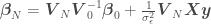
where . Using and assuming a prior of , and then take a new shape in the predictor posterior of a Gaussian Process:
where , and . Now the features of the data are absorbed within the inner-products between observed ‘s and or for , so we can add as many features as we want without impacting the dimensions of the matrix we will have to invert. Also, after this transformation, instead of and representing the mean and covariance between model parameters, they represent the mean and covariance of and among data points and/or points for which we want to get point estimates. The parameter posterior from Bayesian OLR would now be used to sample the values of directly instead of model parameters. And now we have a Gaussian Process with which to estimate . For plots of samples of from the prior and from the predictive posterior, of the mean plus or minus the error variances, and of models with different kernel parameters, see figures at the end of the post.
Kernel (or Covariance) matrices
The convenience of having and written in terms of , is that does not have to represent simply a matrix-matrix or vector-matrix multiplication of and . In fact, function can be any function that corresponds to an inner-product after some transformation from , which will necessarily return a positive semi-definite matrix and therefore be a valid covariance matrix. There are several kernels (or kernel functions or kernel shapes) available, each accounting in a different way for the nearness or similarity (at least in Gaussian Processes) between values of :
the linear kernel: . This kernel is used when trying to fit a line going through the origin.
the polynomial kernel: , where d is the dimension of the polynomial function. This kernel is used when trying to fit a polynomial function (such as the fourth order polynomial in the blog post about Bayesian OLR), and
the Radial Basis Function, or RBF (aka Squared Exponential, or SE), , where is a kernel parameter denoting the characteristic length scale of the function to be approximated. Using the RBF kernel is equivalent to adding an infinite (!) number of features the data, meaning .
But this is all quite algebraic. Luckily, there is a more straight-forward derivation shown next.
Succinct derivation of Gaussian Processes from functional space.
Most regression we study in school is a way of estimating the parameters of a model. In Bayesian OLR, for example, we have a distribution (the parameter posterior) from which to sample model parameters. What if we instead derived a distribution from which to sample functions themselves? The first (and second and third) time I heard about the idea of sampling functions I thought right away of opening a box and from it drawing exponential and sinusoid functional forms. However, what is meant here is a function of an arbitrary shape without functional form. How is this possible? The answer is: instead of sampling a functional form itself, we sample the values of at discrete points, with a collection of for all in our domain called a function . After all, don’t we want a function more often than not solely for the purpose of getting point estimates and associated errors for given values of ?
In Gaussian Process regression, we sample functions from a distribution by considering each value of in a discretized range along the x-axis as a random variable. That means that if we discretize our x-axis range into 100 equally spaced points, we will have 100 random variables . The mean of all possible functions at therefore represents the mean value of in , and each term in the covariance matrix (kernel matrix, see “Kernel (or Covariance) matrices” section above) represents how similar the values of and will be for each pair and based on the value of a distance metric between and : if and are close to each other, and tend to be similar and vice-versa. We can therefore turn the sampled functions into whatever functional form we want by choosing the appropriate covariance matrix (kernel) — e.g. a linear kernel will return a linear model, a polynomial kernel will return a polynomial function, and an RBF kernel will return a function with an all linear and an infinite number of non-linear terms. A Gaussian Process can then be written as
where is the mean function (e.g. a horizontal line along the x-axis at y = 0 would mean that ) and is the covariance matrix, which here expresses how similar the values of will be based on the distance between two values of .
To illustrate this point, assume we want to sample functions over 200 discretizations along the x-axis from x=-5 to x=5 () using a Gaussian Process. Assume the parameters of our Gaussian Process from which we will sample our functions are mean 0 and that it uses an RBF kernel for its covariance matrix with parameter (not be confused with standard deviation), meaning that and , or
Each sample from the normal distribution above will return 200 values: . A draw of 3 such sample functions would look generally like the following:
The functions above look incredibly smooth because of the RBF kernel, which adds an infinite number of non-linear features to the data. The shaded region represents the prior distribution of functions. The grey line in the middle represents the mean of an infinite number of function samples, while the upper and lower bounds represent the corresponding prior mean plus or minus standard deviations.
These functions looks quite nice but pretty useless. We are actually interested in regressing our data assuming a prior, namely on a posterior distribution, not on the prior by itself. Another way of formulating this is to say that we are interested only in the functions that go through or close to certain known values of and . All we have to do is to add random variables corresponding to our data and condition the resulting distribution on them, which means accounting only for samples of functions that exactly go through (or given) our data points. The resulting distribution would then look like . After adding our data , or , our distribution would look like
In this distribution we have random variables representing the from our data set and the from which we want to get point estimates and corresponding error standard deviations. The covariance matrix above accounts for correlations of all observations with all other observations, and correlations of all observations with all points to be predicted. We now just have to condition the multivariate normal distribution above over the points in our data set, so that the distribution accounts for the infinite number of functions that go through our at the corresponding . This yields
where , , , and is a vector containing the elements in the diagonal of the covariance matrix — the variances of each random variable . If you do not want to use a prior with , the mean of the Gaussian Process would be . A plot of estimated for 200 values of — so that the resulting curve looks smooth — plus or minus associated uncertainty (), regressed on 5 random data points , , should look generally like
A plot of three sampled functions (colored lines below, the grey line is the mean) should look generally like
Several kernel have parameters that can strongly influence the regressed model and that can be estimated — see Murphy (2012) for a succinct introduction to kernel parameters estimation. One example is parameter of the RBF kernel, which determines the correlation length scale of the fitted model and therefore how fast with increasing separation distance between data points the model will default to the prior (here, with ). The figure below exemplifies this effect
All figures have the same data points but the resulting models look very different. Reasonable values for depend on the spacing between the data points and are therefore data-specific. Also, if when you saw this plot you thought of fitting RBF functions as interpolators, that was not a coincidence: the equations solved when fitting RBFs to data as interpolators are the same solved when using Gaussian Processes with RBF kernels.
Lastly, in case of noisy observation of in the Gaussian Process distribution and the expressions for the mean, covariance, and standard deviation become
where is the error variance and is an identity matrix. The mean and error predictions would look like the following
Concluding Remarks
What I presented is the very basics of Gaussian Processes, leaving several important topics which were not covered here for the interested reader to look into. Examples are numerically more stable formulations, computationally more efficient formulations, kernel parameter estimation, more kernels, using a linear instead of zero-mean prior (semi-parametric Gaussian Processes), Gaussian Processes for classification and Poisson regression, the connection between Gaussian Processes and other methods, like krieging and kernel methods for nonstationary stochastic processes. Some of these can be found in great detail in Rasmussen and Williams (2006), and Murphy (2012) has a succinct presentation of all of the listed topics.
I was really confused about Gaussian Processes the first time I studied it and tried to make this blog post as accessible as possible. Please leave a comment if you think the post would benefit from any particular clarification.
References
Murphy, Kevin P., 2012. Machine Learning: A Probabilistic Perspective. The MIT Press, ISBN 978-0262018029
Rasmussen, Carl Edward and Williams, Christopher K. I., 2006. Gaussian Processes for Machine Learning. The MIT Press, ISBN 978-0262182539.
In this post, I will briefly review the basic theory about Ordinary Linear Regression (OLR) using the frequentist approach and from it introduce the Bayesian approach. This will lay the terrain for a later post about Gaussian Processes. The reader may ask himself why “Ordinary Linear Regression” instead of “Ordinary Least Squares.” The answer is that least squares refers to the objective function to be minimized, the sum of the square errors, which is not used the Bayesian approach presented here. I want to thank Jared Smith and Jon Lamontagne for reviewing and improving this post. This post closely follows the presentation in Murphy (2012), which for some reason does not use “^” to denote estimated quantities (if you know why, please leave a comment).
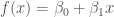
Ordinary Linear Regression
OLR is used to fit a model that is linear in the parameters to a data set , where represents the independent variables and the dependent variable, and has the form
where is a vector of model parameters and is the model error variance. The unusual notation for the normal distribution should be read as “a normal distribution of with (or given) mean and variance .” One frequentist method of estimating the parameters of a linear regression model is the method of maximum likelihood estimation (MLE). MLE provides point estimates for each of the regression model parameters by maximizing the likelihood function with respect to and by solving the maximization problem
where the likelihood function is defined as
where is the mean of the model error (normally ), is the number of points in the data set, is an identity matrix, and is a vector of values of the independent variables for an individual data point of matrix . OLR assumes independence and the same model error variance among observations, which is expressed by the covariance matrix . Digression: in Generalized Linear Regression (GLR), observations may not be independent and may have different variances (heteroscedasticity), so the covariance matrix may have off-diagonal terms and the diagonal terms may not be equal.
If a non-linear function shape is sought, linear regression can be used to fit a model linear in the parameters over a function of the data — I am not sure why the machine learning community chose for this function, but do not confuse it with a normal distribution. This procedure is called basis function expansion and has a likelihood function of the form
where can have, for example, the form
for fitting a parabola to a one-dimensional over . When minimizing the squared residuals we get to the famous Ordinary Least Squares regression. Linear regression can be further developed, for example, into Ridge Regression to better handle multicollinearity by introducing bias to the parameter estimates, and into Kernel Ridge regression to implicitly add non-linear terms to the model. These formulations are beyond the scope of this post.
What is important to notice is that the standard approaches for linear regression described here, although able to fit linear and non-linear functions, do not provide much insight into the model errors. That is when Bayesian methods come to play.
Bayesian Ordinary Linear Regression
In Bayesian Linear regression (and in any Bayesian approach), the parameters are treated themselves as random variables. This allows for the consideration of model uncertainty, given that now instead of having the best point estimates for we have their full distributions from which to sample models — a sample of corresponds to a model. The distribution of parameters , , called the parameter posterior distribution, is calculated by multiplying the likelihood function used in MLE by a prior distribution for the parameters. A prior distribution is assumed from knowledge prior to analyzing new data. In Bayesian Linear Regression, a Gaussian distribution is commonly assumed for the parameters. For example, the prior on can be for algebraic simplicity. The parameter posterior distribution assuming a known then has the form
, given is a constant depending only on the data.
We now have an expression from which to derive our parameter posterior for our linear model from which to sample . If the likelihood and the prior are Gaussian, the parameter posterior will also be a Gaussian, given by
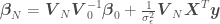
where
If we calculate the parameter posterior (distribution over parameters ) for a simple linear model for a data set in which and are approximately linearly related given some noise , we can use it to sample values for . This is equivalent to sampling linear models for data set . As the number of data points increase, the variability of the sampled models should decrease, as in the figure below
This is all interesting but the parameter posterior per se is not of much use. We can, however, use the parameter posterior to find the posterior predictive distribution, which can be used to both get point estimates of and the associated error. This is done by multiplying the likelihood by the parameter posterior and marginalizing the result over . This is equivalent to performing infinite sampling of blue lines in the example before to form density functions around a point estimate of , with denoting a new point that is not in . If the likelihood and the parameter posterior are Gaussian, the posterior predictive then takes the form below and will also be Gaussian (in Bayesian parlance, this means that the Gaussian distribution is conjugate to itself)!
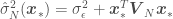
where
or, to put it simply,
The posterior predictive, meaning final linear model and associated errors (the parameter uncertainty equivalent of frequentist statistics confidence intervals) are shown below
If, instead of having a data set in which and are related approximately according to a 4th order polynomial, we use a function to artificially create more random variables (or features, in machine learning parlance) corresponding to the non-linear terms of the polynomial function. Our function would be and the resulting would therefore have five columns instead of two (), so now the task is to find . Following the same logic as before for and , where prime denotes the new set random variable from function , we get the following plots
This looks great, but there is a problem: what if we do not know the functional form of the model we are supposed to fit (e.g. a simple linear function or a 4th order polynomial)? This is often the case, such as when modeling the reliability of a water reservoir system contingent on stored volumes, inflows and evaporation rates, or when modeling topography based on samples surveyed points (we do not have detailed elevation information about the terrain, e.g. a DEM file). Gaussian Processes (GPs) provide a way of going around this difficulty.
References
Murphy, Kevin P., 2012. Machine Learning: A Probabilistic Perspective. The MIT Press.


 for which we are trying to estimate
  with Bayesian OLR is
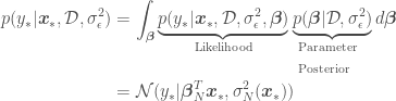
 ,
,  being the independent variables and
  the dependent variable,
  is a vector of model parameters and
  is the model error variance. The unusual notation for the normal distribution
  means “a normal distribution of
  and variance
  ,” where
  is the number of points in the data set. The estimated variance of
  ,
,  can be calculated as
 and
and  are the mean and the covariance of the
 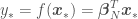 with an error variance of
  ), replace
  and
and  , e.g.
  , to add features to
  , we would instead have that

 and
and  . One problem with this approach is that as we add more terms (also called features) to function
  to better capture non-linearities, the the dimension of the matrix we will have to invert increases. It is also not always obvious what features we should add to our data. Both problems can be handled with Gaussian Processes.
 we have to invert (remember the dimensions of such matrix equals the number of features in

 —
—  is just another point
  either in the data set or for which we want to estimate
  will be called a covariance or kernel function. Since the prior’s covariance
 . Using
  and assuming a prior of
  ,
, 

 ,
,  and
and  . Now the features of the data are absorbed within the inner-products between observed
  ‘s and or for
  , is that
  does not have to represent simply a matrix-matrix or vector-matrix multiplication of
  , which will necessarily return a positive semi-definite matrix and therefore be a valid covariance matrix. There are several kernels (or kernel functions or kernel shapes) available, each accounting in a different way for the nearness or similarity (at least in Gaussian Processes) between values of
  :
: . This kernel is used when trying to fit a line going through the origin.
 , where d is the dimension of the polynomial function. This kernel is used when trying to fit a polynomial function (such as the fourth order polynomial in the blog post about Bayesian OLR), and
 , where
  is a kernel parameter denoting the characteristic length scale of the function to be approximated. Using the RBF kernel is equivalent to adding an infinite (!) number of features the data, meaning
  .
. at discrete points, with a collection of
  for all
  . After all, don’t we want a function more often than not solely for the purpose of getting point estimates and associated errors for given values of
  . The mean of all possible functions at
  in
in  will be for each pair
  based on the value of a distance metric between
  tend to be similar and vice-versa. We can therefore turn the sampled functions
  into whatever functional form we want by choosing the appropriate covariance matrix (kernel) — e.g. a linear kernel will return a linear model, a polynomial kernel will return a polynomial function, and an RBF kernel will return a function with an all linear and an infinite number of non-linear terms. A Gaussian Process can then be written as
 is the mean function (e.g. a horizontal line along the x-axis at y = 0 would mean that
 ![\mu(\boldsymbol{x}) = [0,..,0]^T](https://s0.wp.com/latex.php?latex=%5Cmu%28%5Cboldsymbol%7Bx%7D%29+%3D+%5B0%2C..%2C0%5D%5ET&bg=ffffff&fg=444444&s=0&c=20201002) ) and
) and  along the x-axis from x=-5 to x=5 (
 ) using a Gaussian Process. Assume the parameters of our Gaussian Process from which we will sample our functions are mean 0 and that it uses an RBF kernel for its covariance matrix with parameter
  (not be confused with standard deviation), meaning that
 ![k_{i,i}=1.0 ,\:\forall i \in [0, 199]](https://s0.wp.com/latex.php?latex=k_%7Bi%2Ci%7D%3D1.0+%2C%5C%3A%5Cforall+i+%5Cin+%5B0%2C+199%5D&bg=ffffff&fg=444444&s=0&c=20201002) and
and ![k_{i,j}=e^{-\frac{||x_i-x_j||^2}{2\cdot 2^2}},\: \forall i,j \in [0, 199]](https://s0.wp.com/latex.php?latex=k_%7Bi%2Cj%7D%3De%5E%7B-%5Cfrac%7B%7C%7Cx_i-x_j%7C%7C%5E2%7D%7B2%5Ccdot+2%5E2%7D%7D%2C%5C%3A+%5Cforall+i%2Cj+%5Cin+%5B0%2C+199%5D&bg=ffffff&fg=444444&s=0&c=20201002) , or
, or![\begin{aligned} p(\boldsymbol{f}_*|\boldsymbol{X_*})&=\mathcal{N}(\boldsymbol{f}|\boldsymbol{\mu},\boldsymbol{K_{**}})\\ &=\mathcal{N}\left(\boldsymbol{f}_*\Bigg|[\mu_{*0},..,\mu_{*199}], \begin{bmatrix} k_{*0,0} & k_{*0,1} & \cdots & k_{*0,199} \\ k_{*1,0} & k_{*1, 1} & \cdots & k_{*1,199}\\ \vdots & \vdots & \ddots & \vdots \\ k_{*199,0} & k_{*199,1} & \cdots & k_{*199,199} \end{bmatrix} \right)\\ &=\mathcal{N}\left(\boldsymbol{f}_*\Bigg|[0,..,0], \begin{bmatrix} 1 & 0.9997 & \cdots & 4.2\cdot 10^{-6} \\ 0.9997 & 1 & \cdots & 4.8\cdot 10^{-6}\\ \vdots & \vdots & \ddots & \vdots \\ 4.2\cdot 10^{-6} & 4.8\cdot 10^{-6} & \cdots & 1 \end{bmatrix} \right) \end{aligned}](https://s0.wp.com/latex.php?latex=%5Cbegin%7Baligned%7D+p%28%5Cboldsymbol%7Bf%7D_%2A%7C%5Cboldsymbol%7BX_%2A%7D%29%26%3D%5Cmathcal%7BN%7D%28%5Cboldsymbol%7Bf%7D%7C%5Cboldsymbol%7B%5Cmu%7D%2C%5Cboldsymbol%7BK_%7B%2A%2A%7D%7D%29%5C%5C+%26%3D%5Cmathcal%7BN%7D%5Cleft%28%5Cboldsymbol%7Bf%7D_%2A%5CBigg%7C%5B%5Cmu_%7B%2A0%7D%2C..%2C%5Cmu_%7B%2A199%7D%5D%2C+%5Cbegin%7Bbmatrix%7D+k_%7B%2A0%2C0%7D+%26+k_%7B%2A0%2C1%7D+%26+%5Ccdots+%26+k_%7B%2A0%2C199%7D+%5C%5C+k_%7B%2A1%2C0%7D+%26+k_%7B%2A1%2C+1%7D+%26+%5Ccdots+%26+k_%7B%2A1%2C199%7D%5C%5C+%5Cvdots+%26+%5Cvdots+%26+%5Cddots+%26+%5Cvdots+%5C%5C+k_%7B%2A199%2C0%7D+%26+k_%7B%2A199%2C1%7D+%26+%5Ccdots+%26+k_%7B%2A199%2C199%7D+%5Cend%7Bbmatrix%7D+%5Cright%29%5C%5C+%26%3D%5Cmathcal%7BN%7D%5Cleft%28%5Cboldsymbol%7Bf%7D_%2A%5CBigg%7C%5B0%2C..%2C0%5D%2C+%5Cbegin%7Bbmatrix%7D+1+%26+0.9997+%26+%5Ccdots+%26+4.2%5Ccdot+10%5E%7B-6%7D+%5C%5C+0.9997+%26+1+%26+%5Ccdots+%26+4.8%5Ccdot+10%5E%7B-6%7D%5C%5C+%5Cvdots+%26+%5Cvdots+%26+%5Cddots+%26+%5Cvdots+%5C%5C+4.2%5Ccdot+10%5E%7B-6%7D%C2%A0%26%C2%A04.8%5Ccdot+10%5E%7B-6%7D+%26+%5Ccdots+%26+1+%5Cend%7Bbmatrix%7D+%5Cright%29+%5Cend%7Baligned%7D&bg=ffffff&fg=444444&s=0&c=20201002)
![\boldsymbol{f}_* = [y_0, ..., y_{199}]](https://s0.wp.com/latex.php?latex=%5Cboldsymbol%7Bf%7D_%2A+%3D+%5By_0%2C+...%2C+y_%7B199%7D%5D&bg=ffffff&fg=444444&s=0&c=20201002) . A draw of 3 such sample functions would look generally like the following:
. A draw of 3 such sample functions would look generally like the following:
 . All we have to do is to add random variables corresponding to our data and condition the resulting distribution on them, which means accounting only for samples of functions that exactly go through (or given) our data points. The resulting distribution would then look like
  . After adding our data
  , or
, or  , our distribution would look like
 from which we want to get point estimates and corresponding error standard deviations. The covariance matrix above accounts for correlations of all observations with all other observations, and correlations of all observations with all points to be predicted. We now just have to


 ,
,  ,
,  , and
, and  is a vector containing the elements in the diagonal of the covariance matrix
  — the variances
  of each random variable
 ![\boldsymbol{\mu} = \boldsymbol{\mu}_* = [0, ... , 0]^T](https://s0.wp.com/latex.php?latex=%5Cboldsymbol%7B%5Cmu%7D+%3D+%5Cboldsymbol%7B%5Cmu%7D_%2A+%3D+%5B0%2C+...+%2C+0%5D%5ET&bg=ffffff&fg=444444&s=0&c=20201002) , the mean of the Gaussian Process would be
, the mean of the Gaussian Process would be  . A plot of
  estimated for 200 values of
  ), regressed on 5 random data points
 should look generally like
 of the RBF kernel, which determines the correlation length scale of the fitted model and therefore how fast with increasing separation distance between data points the model will default to the prior (here, with
  ). The figure below exemplifies this effect


 and variance
  for each of the regression model parameters
 is defined as
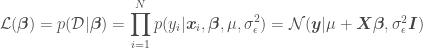
 is the mean of the model error (normally
  ),
),  . Digression: in Generalized Linear Regression (GLR), observations may not be independent and may have different variances (heteroscedasticity), so the covariance matrix may have off-diagonal terms and the diagonal terms may not be equal.
 for this function, but do not confuse it with a normal distribution. This procedure is called basis function expansion and has a likelihood function of the form

 , called the parameter posterior distribution, is calculated by multiplying the likelihood function used in MLE by a prior distribution for the parameters. A prior distribution is assumed from knowledge prior to analyzing new data. In Bayesian Linear Regression, a Gaussian distribution is commonly assumed for the parameters. For example, the prior on
  for algebraic simplicity. The parameter posterior distribution assuming a known
  , given
  is a constant depending only on the data.

 for a data set
  for data set
 , with
  denoting a new point that is not in
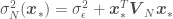


![\phi(x) = [1, x, x^2, x^3, x^4]^T](https://s0.wp.com/latex.php?latex=%5Cphi%28x%29+%3D+%5B1%2C+x%2C+x%5E2%2C+x%5E3%2C+x%5E4%5D%5ET&bg=ffffff&fg=444444&s=0&c=20201002) and the resulting
and the resulting  would therefore have five columns instead of two (
![[1, x]^T](https://s0.wp.com/latex.php?latex=%5B1%2C+x%5D%5ET&bg=ffffff&fg=444444&s=0&c=20201002) ), so now the task is to find
), so now the task is to find ![\boldsymbol{\beta}=[\beta_0, \beta_1, \beta_2, \beta_3, \beta_4]^T](https://s0.wp.com/latex.php?latex=%5Cboldsymbol%7B%5Cbeta%7D%3D%5B%5Cbeta_0%2C+%5Cbeta_1%2C+%5Cbeta_2%2C+%5Cbeta_3%2C+%5Cbeta_4%5D%5ET&bg=ffffff&fg=444444&s=0&c=20201002) . Following the same logic as before for
. Following the same logic as before for  and
and  , where prime denotes the new set random variable
  from function

