
You are probably asking yourself “and why do I need more terminal schooling?”. The short answer is: to not have to spend as much time as you do on the terminal, most of which spent (1) pushing arrow keys thousands of times per afternoon to move through a command or history of commands, (2) waiting for a command that takes forever to be done running before you can run anything else, (3) clicking all over the place on MobaXTerm and still feeling lost, (4) manually running the same command multiple times with different inputs, (5) typing the two-step verification token every time you want to change a “+” to a “-” on a file on a supercomputer, (6) waiting forever for a time-consuming run done in serial on a single core, and (7, 8, …) other useless and horribly frustrating chores. Below are some tricks to make your Linux work more efficient and reduce the time you spend on the terminal. From now on, I will use a “$” sign to indicate that what follows is a command typed in the terminal.
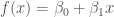
The tab autocomple is your best friend
When trying to do something with that file whose name is 5480458 characters long, be smart and don’t type the whole thing. Just type the first few letters and hit tab. If it doesn’t complete all the way it’s because there are multiple files whose names begin with the sequence of characters. In this case, hitting tab twice will return the names of all such files. The tab autocomplete works for commands as well.
Ctrl+r for search through previous commands
When on the terminal, hit ctrl+r to switch to reverse search mode. This works like a simple search function o a text document, but instead looking in your bash history file for commands you used over the last weeks or months. For example, if you hit ctrl+r and type sbatch it will fill the line with the last command you ran that contained the word sbatch. If you hit ctrl+r again, it will find the second last used command, and so on.
Vim basics to edit files on a system that requires two-step authentication
Vim is one the most useful things I have came across when it comes to working on supercomputers with two-step identity verification, in which case using MobaXTerm of VS Code requires typing a difference security code all the time. Instead of uploading a new version of a code file every time you want to make a simple change, just edit the file on the computer itself using Vim. To make simple edits on your files, there are very few commands you need to know.
To open a file with Vim from the terminal: $ vim <file name> or $ vim +10 <file name>, if you want to open the file and go straight to line 10.
Vim has two modes of operation: text-edit (for you to type whatever you want in the file) and command (replacement to clicking on file, edit, view, etc. on the top bar of notepad). When you open Vim, it will be in command mode.
To switch to text-edit mode, just hit either “a” or “i” (you should then see “– INSERT –” at the bottom of the screen). To return to command mode, hit escape (Esc). When in text-edit more, the keys “Home,” “End,” “Pg Up,” “Pg Dn,” “Backspace,” and “Delete” work just like on Notepad and MS Word.
When in command mode, save your file by typing :w + Enter, save and quite with :wq, and quit without saving with :q!. Commands for selecting, copying and pasting, finding and replacing, replacing just one character, deleting a line, and other more advanced tasks can be found here. There’s also a great cheatsheet for Vim here. Hint: once you learn some more five to ten commands, making complex edits on your file with Vim becomes blazingly fast.
Perform repetitive tasks on the terminal using one-line Bash for-loops.
Instead of manually typing a command for each operation you want to perform on a subset of files in a directory (“e.g., cp file<i>.csv directory300-400 for i from 300 to 399 , tar -xzvf myfile<i>.tar.gz, etc.), you can use a Bash for-loop if using the is not possible.
Consider a situation in which you have 10,000 files and want to move files number 200 to 299 to a certain directory. Using the wildcard “*” in this case wouldn’t be possible, as result_2<i>.csv would return result_2.csv, result_20.csv to result_29.csv, and result_2000.csv to result_2999.csv as well–sometimes you may be able to use Regex, but that’s another story. To move a subset of result files to a directory using a Bash for-loop, you can use the following syntax:
$ for i in {0..99}; do cp result_2$i results_200s/; done
Keep in mind that you can have multiple commands inside a for-loop by separating them with “;” and also nest for-loops.
Run a time-intensive command on the background with an “&” and keep doing your terminal work
Some commands may take a long time to run and render the terminal unusable until it’s complete. Instead of opening another instance of the terminal and login in again, you can send a command to the background by adding “&” at the end of it. For example, if you want to extract a tar file with dozens of thousands of files in it and keep doing your work as the files are extracted, just run:
$ tar -xzf my_large_file.tar.gz &
If you have a directory with several tar files and want to extract a few of them in parallel while doing your work, you can use the for-loop described above and add “&” to the end of the tar command inside the loop. BE CAREFUL, if your for-loop iterates over dozens or more files, you may end up with your terminal trying to run dozens or more tasks at once. I accidentally crashed the Cube once doing this.
Check what is currently running on the terminal using ps
To make sure you are not overloading the terminal by throwing too many processes at it, you can check what it is currently running by running the command ps. For example, if I run an program with MPI creating two processes and run ps before my program is done, it will return the following:
bernardoct@DESKTOP-J6145HK /mnt/c/Users/Bernardo/CLionProjects/WaterPaths
$ mpirun -n 2 ./triangleSimulation -I Tests/test_input_file_borg.wp &
[1] 6129     <-- this is the process ID
bernardoct@DESKTOP-J6145HK /mnt/c/Users/Bernardo/CLionProjects/WaterPaths
 $ ps
 PID TTY TIME CMD
 8 tty1 00:00:00 bash
 6129 tty1 00:00:00 mpirun    <-- notice the process ID 6129 again
 6134 tty1 00:00:00 triangleSimulat
 6135 tty1 00:00:00 triangleSimulat
 6136 tty1 00:00:00 ps
Check the output of a command running on the background
If you run a program on the background its output will not be printed on the screen. To know what’s happening with your program, send (to pipe) its output to a text file using the “>” symbol, which will be updated continuously as your program is running, and check it with cat <file name>, less +F, <file name>tail -n, or something similar. For example, if test_for_background.sh is a script that will print a number on the screen every one second, you could do the following (note the “> pipe.csv” in the first command):<file name>
bernardoct@DESKTOP-J6145HK /mnt/c/Users/Bernardo/CLionProjects/WaterPaths
 $ ./test_for_background.sh > pipe.csv &
 [1] 6191

bernardoct@DESKTOP-J6145HK /mnt/c/Users/Bernardo/CLionProjects/WaterPaths
 $ cat pipe.csv
 1
 2

bernardoct@DESKTOP-J6145HK /mnt/c/Users/Bernardo/CLionProjects/WaterPaths
 $ cat pipe.csv
 1
 2
 3

bernardoct@DESKTOP-J6145HK /mnt/c/Users/Bernardo/CLionProjects/WaterPaths
 $ tail -3 pipe.csv
 8
 9
 10
This is also extremely useful in situations when you want to run a command that takes long to run but whose outputs are normally displayed one time on the screen. For example, if you want to check the contents of a directory with thousands of files to search for a few specific files, you can pipe the output of ls to a file and send it to the background with ls > directory_contents.txt & and search the resulting text file for the file of interest.
System monitor: check core and memory usage with htop, or top if htop is not available
If ps does not provide enough information given your needs, such as if you’re trying to check if your multi-thread application is using the number of cores it should, you can try running htop instead. This will show on your screen something along the lines of the Performance view of Windows’ Task Manager, but without the time plot. It will also show how much memory is being used, so that you do not accidentally shut down a node on an HPC system. If htop is not available, you can try top.
Running make in parallel with make -j for much shorter compiling time
If a C++ code is properly modularized, make can compile certain source code files in parallel. To do that, run make -j<number of cores> <rule in makefile>. For example, the following command would compile WaterPaths in parallel over four cores:
$ make -j4 gcc
For WaterPaths, make gcc takes 54s on the Cube, make -j4 gcc takes 15s, make -j8 gcc takes 9s, so the time and patience savings are real if you have to compile the code various times per day. To make your life simpler, you can add an alias to bash_aliases such as alias make='make -j4' (see below in section about .bash_aliases file). DO NOT USE MAKE -J ON NSF HPC SYSTEMS: it is against the rules. On the cube keep it to four cores or less not to disturb other users, but use all cores available if on the cloud or iterative section.
Check the size of files and directories using du -hs
The title above is quite self-explanatory. Running du -hs <file name> will tell you its size.
Check the data and time a file was created or last modified using the stat command
Also rather self-explanatory. Running stat <file name> is really useful if you cannot remember on which file you saved the output last time you ran your program.
Split large files into smaller chunks with the split command and put them back together with cat
This works for splitting a large text file into files with fewer lines, as well as for splitting large binary files (such as large tar files) so that you can, for example, upload them to GitHub or e-mail them to someone. To split a text file with 10,000 into ten files with 1,000 lines each, use:
$ split -l 1000 myfile myfile_part
This will result in ten files called myfile_part00, myfile_part01, and so on with 1,000 lines each. Similarly, the command below would break a binary file into parts with 50 MB each:
$ split -b 50m myfile myfile_part
To put all files back together in either case, run:
$ cat myfile_part* myfile
More information about the split command can be found in Joe’s post about it.
Checking your HPC submission history with `sacct`
Another quite sulf-explanatory tile. If you want to remember when you submitted something, such as to check if an output file resulted from this or that submission (see stat command), just run the command below in one line:
$ sacct -S 2019-09-18 -u bct52 --format=User,JobID,Jobname,start,end,elapsed,nnodes,nodelist,state
This will result in an output similar to the one below:
bct52 979 my_job 2019-09-10T21:48:30 2019-09-10T21:55:08 00:06:38 1 c0001 COMPLETED
bct52 980 skx_test_1 2019-09-11T01:44:08 2019-09-11T01:44:09 00:00:01 1 c0001 FAILED
bct52 981 skx_test_1 2019-09-11T01:44:33 2019-09-11T01:56:45 00:12:12 1 c0001 CANCELLED
bct52 1080 skx_test_4 2019-09-11T22:07:03 2019-09-11T22:08:39 00:01:36 4 c[0001-0004] COMPLETED
1080.0 orted 2019-09-11T22:08:38 2019-09-11T22:08:38 00:00:00 3 c[0002-0004] COMPLETED
Compare files with meld, fldiff, or diff
There are several programs to show the differences between text files. This is particularly useful when you want to see what the changes between different versions of the same file, normally a source code file. If you are on a computer running a Linux OS or have an X server like Xming installed, you can use meld and kdiff3 for pretty outputs on a nice GUI or fldiff to quickly handle a files with huge number of difference. Otherwise, diff will show you the differences in a cruder pure-terminal but still very much functional manner. The syntax for all of them is:
$ <command> <file1> <file2>
Except for diff, for which it is worth calling with the --color option:
$ diff --color <file1> <file2>
If cannot run a graphical user interface but is feeling fancy today, you can install the ydiff Python extension with (done just once):
$ python3 -m pip install --user ydiff
and pipe diff’s output to it with the following:
$diff -u <file1> <file2> | python3 -m ydiff -s
This will show you the differences between two versions of a code file in a crystal clear, side by side, and colorized way.
Creating a .bashrc file for a terminal that’s easy to work with and good (or better) to look at
When we first login to several Linux systems the terminal is all black with white characters, in which it’s difficult find the commands you typed amidst all the output printed on the screen, and with limited autocomplete and history search. In short, it’s a real pain and you makes you long for Windows as much as for you long for your mother’s weekend dinner. There is, however, a way of making the terminal less of a pain to work with, which is by creating a file called .bashrc with the right contents in your home directory. Below is an example of a .bashrc file with the following features for you to just copy and paste in your home directory (e.g., /home/username/, or ~/ for short):
- Colorize your username and show the directory you’re currently in, so that it’s easy to see when the output of a command ends and the next one begins–as in section “Checking the output of a command running on the background.”
- Allow for a search function with the up and down arrow keys. This way, if you’re looking for all the times you typed a command starting with sbatch, you can just type “sba” and hit up arrow until you find the call you’re looking for.
- A function that allows you to call extract and the compressed file will be extracted. No more need to tar with a bunch of options, unzip, unrar, etc. so long as you have all of them installed.
- Colored man pages. This means that when you look for the documentation of a program using man, such as man cat to see all available options for the cat command, the output will be colorized.
- A function called pretty_csv to let you see csv files in a convenient, organized and clean way from the terminal, without having to download it to your computer.
# .bashrc

# Source global definitions
if [ -f /etc/bashrc ]; then
. /etc/bashrc
fi

# Load aliases
if [ -f ~/.bash_aliases ]; then
. ~/.bash_aliases
fi

# Automatically added by module
shopt -s expand_aliases

if [ ! -z "$PS1" ]; then
PS1='\[\033[G\]\[\e]0;\w\a\]\n\[\e[1;32m\]\u@\h \[\e[33m\]\w\[\e[0m\]\n\$ '
bind '"\e[A":history-search-backward'
bind '"\e[B":history-search-forward'
fi

set show-all-if-ambiguous on
set completion-ignore-case on
export PATH=/usr/local/gcc-7.1/bin:$PATH
export LD_LIBRARY_PATH=/usr/local/gcc-7.1/lib64:$LD_LIBRARY_PATH

history -a
export DISPLAY=localhost:0.0

sshd_status=$(service ssh status)
if [[ $sshd_status = *"is not running"* ]]; then
sudo service ssh --full-restart
fi

HISTSIZE=-1
HISTFILESIZE=-1

extract () {
if [ -f $1 ] ; then
case $1 in
*.tar.bz2)   tar xvjf $1    ;;
*.tar.gz)    tar xvzf $1    ;;
*.bz2)       bunzip2 $1     ;;
*.rar)       unrar x $1       ;;
*.gz)        gunzip $1      ;;
*.tar)       tar xvf $1     ;;
*.tbz2)      tar xvjf $1    ;;
*.tgz)       tar xvzf $1    ;;
*.zip)       unzip $1       ;;
*.Z)         uncompress $1  ;;
*.7z)        7z x $1        ;;
*)           echo "don't know how to extract '$1'..." ;;
esac
else
echo "'$1' is not a valid file!"
fi
}

# Colored man pages
export LESS_TERMCAP_mb=$'\E[01;31m'
export LESS_TERMCAP_md=$'\E[01;31m'
export LESS_TERMCAP_me=$'\E[0m'
export LESS_TERMCAP_se=$'\E[0m'
export LESS_TERMCAP_so=$'\E[01;44;33m'
export LESS_TERMCAP_ue=$'\E[0m'
export LESS_TERMCAP_us=$'\E[01;32m'

# Combine multiline commands into one in history
shopt -s cmdhist

# Ignore duplicates, ls without options and builtin commands
HISTCONTROL=ignoredups
export HISTIGNORE="&:ls:[bf]g:exit"

pretty_csv () {
cat "$1" | column -t -s, | less -S
}
There are several .bashrc example files online with all sorts of functionalities. Believe me, a nice .bashrc will make your life A LOT BETTER. Just copy and paste the above into a text file called .bashrc and sent it to your home directory in your local or HPC system terminal.
Make the terminal far less user-friendly and less archane by setting up a .bash_aliases file
You should also have a .bash_aliases file to significantly reduce typing and colorizing the output of commands you often use for ease of navigation. Just copy all the below into a file called .bash_aliases and copy into your home directory (e.g., /home/username/, or ~/ for short). This way, every time you run the command between the word “alias” and the “=” sign, the command after the “=”sign will be run.
alias ls='ls --color=tty'
alias ll='ls -l --color=auto'
alias lh='ls -al --color=auto'
alias lt='ls -alt --color=auto'
alias uu='sudo apt-get update && sudo apt-get upgrade -y'
alias q='squeue -u '
alias qkill='scancel $(qselect -u bct52)'
alias csvd="awk -F, 'END {printf \"Number of Rows: %s\\nNumber of Columns: %s\\n\", NR, NF}'"
alias grep='grep --color=auto'                          #colorize grep output
alias gcc='gcc -fdiagnostics-color=always'                           #colorize gcc output
alias g++='g++ -fdiagnostics-color=always'                          #colorize g++ output
alias paper='cd /my/directory/with/my/beloved/paper/'
alias res='cd /my/directory/with/my/ok/results/'
alias diss='cd /my/directory/of/my/@#$%&/dissertation/'
alias aspell='aspell --lang=en --mode=tex check'
alias aspellall='find . -name "*.tex" -exec aspell --lang=en --mode=tex check "{}" \;'
alias make='make -j4'
Check for spelling mistakes in your Latex files using aspell
Command-line spell checker, you know what this is.
aspell --lang=en --mode=tex check'
To run aspell check on all the Latexfiles in a directory and its subdirectories, run:
find . -name "*.tex" -exec aspell --lang=en --mode=tex check "{}" \;
Easily share a directory on certain HPC systems with others working on the same project [Hint from Stampede 2]
Here’s a great way to set permissions recursively to share a directory named projdir with your research group:
$ lfs find projdir | xargs chmod g+rX
Using lfs is faster and less stressful on Lustre than a recursive chmod. The capital “X” assigns group execute permissions only to files and directories for which the owner has execute permissions.
Run find and replace in all files in a directory [Hint from Stampede 2]
Suppose you wish to remove all trailing blanks in your *.c and *.h files. You can use the find command with the sed command with in place editing and regular expressions to this. Starting in the current directory you can do:
$ find . -name *.[ch] -exec sed -i -e ‘s/ +$//’ {} \;
The find command locates all the *.c and *.h files in the current directory and below. The -exec option run the sed command replacing {} with the name of each file. The -i option tells sed to make the changes in place. The s/ +$// tells sed to replace one or blanks at the end of the line with nothing. The \; is required to let find know where the end of the text for the -exec option. Being an effective user of sed and find can make a great different in your productivity, so be sure to check Tina’s post about them.
Other post in this blog
Be sure to look at other posts in this blog, such as Jon Herman’s post about ssh, Bernardo’s post about other useful Linux commands organized by task to be performed, and Joe’s posts about grep (search inside multiple files) and cut.


 is the weight assigned to weak classifier
  around samples
  at iteration t, and T is the number of classifiers in the ensemble.
 is a loss function, Boosting is trained via gradient descent in functional space, so that:

 to the value of
  with the minimum value of
  , which in machine learning is a loss function, henceforth called
  . Gradient descent does that by moving one step of length s at a time starting from
  in the direction of the steeped downhill slope at location
  , the value of
  iteration. This idea is formalized by the Taylor series expansion below:
 . Furthermore,
![\ell\left[x_{t+1} -\alpha g(x_t)\right] \approx \ell(x^{t})-\alpha g(x_t)^Tg(x_t)](https://s0.wp.com/latex.php?latex=%5Cell%5Cleft%5Bx_%7Bt%2B1%7D+-%5Calpha+g%28x_t%29%5Cright%5D+%5Capprox+%5Cell%28x%5E%7Bt%7D%29-%5Calpha+g%28x_t%29%5ETg%28x_t%29&bg=ffffff&fg=444444&s=0&c=20201002)
 , called the learning rate, must be positive and can be set as a fixed parameter. The dot product on the last term
  will also always be positive, which means that the loss should always decrease — the reason for the italics is that too high values for
  would be a function of a function, say
  instead of a real number x. As mentioned, Gradient Descent in real space works by adding small quantities to
  , which is an ensemble of small
  ‘s added together. By analogy, gradient descent in functional space works by adding functions to an ever growing ensemble of functions. Using the definition of a functional gradient, which is beyond the scope of the this post, this leads us to:
 notation denotes a dot product between f and g. Gradient descent in function space is an important component of Boosting. Based on that, the next section will talk about AdaBoost, a specific Boosting algorithm.
 is the
  data point in the training set. The step size
  have corresponding vector of dependent variables
  , in which each
  is a vector with the classification of each point, with -1 and 1 representing the two classes to which a point may belong (say, -1 for red circles and 1 for blue crosses). The weak classifiers h in AdaBoost also return
  .
.
![\alpha=argmin_{\alpha}\sum_{i=1}^ne^{y(\boldsymbol{x}_i)\left[H(\boldsymbol{x}_i)+\alpha h(\boldsymbol{x}_i)\right]}](https://s0.wp.com/latex.php?latex=%5Calpha%3Dargmin_%7B%5Calpha%7D%5Csum_%7Bi%3D1%7D%5Ene%5E%7By%28%5Cboldsymbol%7Bx%7D_i%29%5Cleft%5BH%28%5Cboldsymbol%7Bx%7D_i%29%2B%5Calpha+h%28%5Cboldsymbol%7Bx%7D_i%29%5Cright%5D%7D+&bg=ffffff&fg=444444&s=0&c=20201002)

 is the classification error of weak classifier
  will be the one that minimizes the term
  , which when zero would mean that the zero-slope ensemble has been reached, denoting the minimum value of the loss function has been reached for a convex problem such as this. Replacing the dot product by a summation, this minimization problem can be written as:


 — e.g., in panel “b” the error would be summation the of the weights of the two crosses on the upper left corner and of the circle at the bottom right corner. Now let’s get to these weights.
 is a vector containing the weights of each point, Z is a normalization factor to ensure the weights will sum up to 1. Be sure not to confuse
  . For the weights to sum up to 1, Z needs to be the sum of their pre-normalization values, which is actually identical to the loss function, so


 . We have that:
![\ell(H)\leq n\left[2\sqrt{\epsilon_{max}(1-\epsilon_{max})}\right]^T](https://s0.wp.com/latex.php?latex=%5Cell%28H%29%5Cleq+n%5Cleft%5B2%5Csqrt%7B%5Cepsilon_%7Bmax%7D%281-%5Cepsilon_%7Bmax%7D%29%7D%5Cright%5D%5ET+&bg=ffffff&fg=444444&s=0&c=20201002)
 , we have that

 in the interval
 ![\left[-\frac{1}{2},\frac{1}{2}\right]](https://s0.wp.com/latex.php?latex=%5Cleft%5B-%5Cfrac%7B1%7D%7B2%7D%2C%5Cfrac%7B1%7D%7B2%7D%5Cright%5D&bg=ffffff&fg=444444&s=0&c=20201002) . Therefore, replacing the equation above in the first loss inequality written as a function of
. Therefore, replacing the equation above in the first loss inequality written as a function of 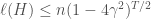
 regularization, which is prone to eliminate irrelevant features and thus reduce overfitting. Another explanation is related to the concept of margins, so that at least certain boosting algorithms force a classification on a point only if possible by a certain margin, thus also preventing overfitting.
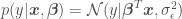
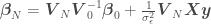
 for which we are trying to estimate
  with Bayesian OLR is
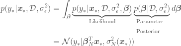
 ,
,  being the independent variables and
  the dependent variable,
  is a vector of model parameters and
  is the model error variance. The unusual notation for the normal distribution
  means “a normal distribution of
  and variance
  ,” where
  is the number of points in the data set. The estimated variance of
  ,
,  can be calculated as
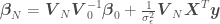
 and
and  are the mean and the covariance of the
  with an error variance of
  ), replace
  and
and  , e.g.
  , to add features to
  , we would instead have that

 and
and  . One problem with this approach is that as we add more terms (also called features) to function
  to better capture non-linearities, the the dimension of the matrix we will have to invert increases. It is also not always obvious what features we should add to our data. Both problems can be handled with Gaussian Processes.
 we have to invert (remember the dimensions of such matrix equals the number of features in

 —
—  is just another point
  either in the data set or for which we want to estimate
  will be called a covariance or kernel function. Since the prior’s covariance
 . Using
  and assuming a prior of
  ,
, 

 ,
,  and
and  . Now the features of the data are absorbed within the inner-products between observed
  , is that
  does not have to represent simply a matrix-matrix or vector-matrix multiplication of
  , which will necessarily return a positive semi-definite matrix and therefore be a valid covariance matrix. There are several kernels (or kernel functions or kernel shapes) available, each accounting in a different way for the nearness or similarity (at least in Gaussian Processes) between values of
  :
: . This kernel is used when trying to fit a line going through the origin.
 , where d is the dimension of the polynomial function. This kernel is used when trying to fit a polynomial function (such as the fourth order polynomial in the blog post about Bayesian OLR), and
 , where
  is a kernel parameter denoting the characteristic length scale of the function to be approximated. Using the RBF kernel is equivalent to adding an infinite (!) number of features the data, meaning
  .
. at discrete points, with a collection of
  for all
  . After all, don’t we want a function more often than not solely for the purpose of getting point estimates and associated errors for given values of
  . The mean of all possible functions at
  in
in  will be for each pair
  based on the value of a distance metric between
  tend to be similar and vice-versa. We can therefore turn the sampled functions
  into whatever functional form we want by choosing the appropriate covariance matrix (kernel) — e.g. a linear kernel will return a linear model, a polynomial kernel will return a polynomial function, and an RBF kernel will return a function with an all linear and an infinite number of non-linear terms. A Gaussian Process can then be written as
 is the mean function (e.g. a horizontal line along the x-axis at y = 0 would mean that
 ![\mu(\boldsymbol{x}) = [0,..,0]^T](https://s0.wp.com/latex.php?latex=%5Cmu%28%5Cboldsymbol%7Bx%7D%29+%3D+%5B0%2C..%2C0%5D%5ET&bg=ffffff&fg=444444&s=0&c=20201002) ) and
) and  along the x-axis from x=-5 to x=5 (
 ) using a Gaussian Process. Assume the parameters of our Gaussian Process from which we will sample our functions are mean 0 and that it uses an RBF kernel for its covariance matrix with parameter
  (not be confused with standard deviation), meaning that
 ![k_{i,i}=1.0 ,\:\forall i \in [0, 199]](https://s0.wp.com/latex.php?latex=k_%7Bi%2Ci%7D%3D1.0+%2C%5C%3A%5Cforall+i+%5Cin+%5B0%2C+199%5D&bg=ffffff&fg=444444&s=0&c=20201002) and
and ![k_{i,j}=e^{-\frac{||x_i-x_j||^2}{2\cdot 2^2}},\: \forall i,j \in [0, 199]](https://s0.wp.com/latex.php?latex=k_%7Bi%2Cj%7D%3De%5E%7B-%5Cfrac%7B%7C%7Cx_i-x_j%7C%7C%5E2%7D%7B2%5Ccdot+2%5E2%7D%7D%2C%5C%3A+%5Cforall+i%2Cj+%5Cin+%5B0%2C+199%5D&bg=ffffff&fg=444444&s=0&c=20201002) , or
, or![\begin{aligned} p(\boldsymbol{f}_*|\boldsymbol{X_*})&=\mathcal{N}(\boldsymbol{f}|\boldsymbol{\mu},\boldsymbol{K_{**}})\\ &=\mathcal{N}\left(\boldsymbol{f}_*\Bigg|[\mu_{*0},..,\mu_{*199}], \begin{bmatrix} k_{*0,0} & k_{*0,1} & \cdots & k_{*0,199} \\ k_{*1,0} & k_{*1, 1} & \cdots & k_{*1,199}\\ \vdots & \vdots & \ddots & \vdots \\ k_{*199,0} & k_{*199,1} & \cdots & k_{*199,199} \end{bmatrix} \right)\\ &=\mathcal{N}\left(\boldsymbol{f}_*\Bigg|[0,..,0], \begin{bmatrix} 1 & 0.9997 & \cdots & 4.2\cdot 10^{-6} \\ 0.9997 & 1 & \cdots & 4.8\cdot 10^{-6}\\ \vdots & \vdots & \ddots & \vdots \\ 4.2\cdot 10^{-6} & 4.8\cdot 10^{-6} & \cdots & 1 \end{bmatrix} \right) \end{aligned}](https://s0.wp.com/latex.php?latex=%5Cbegin%7Baligned%7D+p%28%5Cboldsymbol%7Bf%7D_%2A%7C%5Cboldsymbol%7BX_%2A%7D%29%26%3D%5Cmathcal%7BN%7D%28%5Cboldsymbol%7Bf%7D%7C%5Cboldsymbol%7B%5Cmu%7D%2C%5Cboldsymbol%7BK_%7B%2A%2A%7D%7D%29%5C%5C+%26%3D%5Cmathcal%7BN%7D%5Cleft%28%5Cboldsymbol%7Bf%7D_%2A%5CBigg%7C%5B%5Cmu_%7B%2A0%7D%2C..%2C%5Cmu_%7B%2A199%7D%5D%2C+%5Cbegin%7Bbmatrix%7D+k_%7B%2A0%2C0%7D+%26+k_%7B%2A0%2C1%7D+%26+%5Ccdots+%26+k_%7B%2A0%2C199%7D+%5C%5C+k_%7B%2A1%2C0%7D+%26+k_%7B%2A1%2C+1%7D+%26+%5Ccdots+%26+k_%7B%2A1%2C199%7D%5C%5C+%5Cvdots+%26+%5Cvdots+%26+%5Cddots+%26+%5Cvdots+%5C%5C+k_%7B%2A199%2C0%7D+%26+k_%7B%2A199%2C1%7D+%26+%5Ccdots+%26+k_%7B%2A199%2C199%7D+%5Cend%7Bbmatrix%7D+%5Cright%29%5C%5C+%26%3D%5Cmathcal%7BN%7D%5Cleft%28%5Cboldsymbol%7Bf%7D_%2A%5CBigg%7C%5B0%2C..%2C0%5D%2C+%5Cbegin%7Bbmatrix%7D+1+%26+0.9997+%26+%5Ccdots+%26+4.2%5Ccdot+10%5E%7B-6%7D+%5C%5C+0.9997+%26+1+%26+%5Ccdots+%26+4.8%5Ccdot+10%5E%7B-6%7D%5C%5C+%5Cvdots+%26+%5Cvdots+%26+%5Cddots+%26+%5Cvdots+%5C%5C+4.2%5Ccdot+10%5E%7B-6%7D%C2%A0%26%C2%A04.8%5Ccdot+10%5E%7B-6%7D+%26+%5Ccdots+%26+1+%5Cend%7Bbmatrix%7D+%5Cright%29+%5Cend%7Baligned%7D&bg=ffffff&fg=444444&s=0&c=20201002)
![\boldsymbol{f}_* = [y_0, ..., y_{199}]](https://s0.wp.com/latex.php?latex=%5Cboldsymbol%7Bf%7D_%2A+%3D+%5By_0%2C+...%2C+y_%7B199%7D%5D&bg=ffffff&fg=444444&s=0&c=20201002) . A draw of 3 such sample functions would look generally like the following:
. A draw of 3 such sample functions would look generally like the following:
 . All we have to do is to add random variables corresponding to our data and condition the resulting distribution on them, which means accounting only for samples of functions that exactly go through (or given) our data points. The resulting distribution would then look like
  . After adding our data
  , or
, or  , our distribution would look like
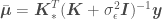
 from which we want to get point estimates and corresponding error standard deviations. The covariance matrix above accounts for correlations of all observations with all other observations, and correlations of all observations with all points to be predicted. We now just have to


 ,
,  ,
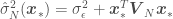
,  , and
, and  is a vector containing the elements in the diagonal of the covariance matrix
  — the variances
  of each random variable
 ![\boldsymbol{\mu} = \boldsymbol{\mu}_* = [0, ... , 0]^T](https://s0.wp.com/latex.php?latex=%5Cboldsymbol%7B%5Cmu%7D+%3D+%5Cboldsymbol%7B%5Cmu%7D_%2A+%3D+%5B0%2C+...+%2C+0%5D%5ET&bg=ffffff&fg=444444&s=0&c=20201002) , the mean of the Gaussian Process would be
, the mean of the Gaussian Process would be  . A plot of
  estimated for 200 values of
  ), regressed on 5 random data points
 should look generally like
 of the RBF kernel, which determines the correlation length scale of the fitted model and therefore how fast with increasing separation distance between data points the model will default to the prior (here, with
  ). The figure below exemplifies this effect


 and variance
  for each of the regression model parameters
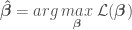
 is defined as
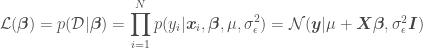
 is the mean of the model error (normally
  ),
),  . Digression: in Generalized Linear Regression (GLR), observations may not be independent and may have different variances (heteroscedasticity), so the covariance matrix may have off-diagonal terms and the diagonal terms may not be equal.
 for this function, but do not confuse it with a normal distribution. This procedure is called basis function expansion and has a likelihood function of the form

 , called the parameter posterior distribution, is calculated by multiplying the likelihood function used in MLE by a prior distribution for the parameters. A prior distribution is assumed from knowledge prior to analyzing new data. In Bayesian Linear Regression, a Gaussian distribution is commonly assumed for the parameters. For example, the prior on
  for algebraic simplicity. The parameter posterior distribution assuming a known
  , given
  is a constant depending only on the data.

 for a data set
 , with
  denoting a new point that is not in
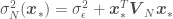


![\phi(x) = [1, x, x^2, x^3, x^4]^T](https://s0.wp.com/latex.php?latex=%5Cphi%28x%29+%3D+%5B1%2C+x%2C+x%5E2%2C+x%5E3%2C+x%5E4%5D%5ET&bg=ffffff&fg=444444&s=0&c=20201002) and the resulting
and the resulting  would therefore have five columns instead of two (
![[1, x]^T](https://s0.wp.com/latex.php?latex=%5B1%2C+x%5D%5ET&bg=ffffff&fg=444444&s=0&c=20201002) ), so now the task is to find
), so now the task is to find ![\boldsymbol{\beta}=[\beta_0, \beta_1, \beta_2, \beta_3, \beta_4]^T](https://s0.wp.com/latex.php?latex=%5Cboldsymbol%7B%5Cbeta%7D%3D%5B%5Cbeta_0%2C+%5Cbeta_1%2C+%5Cbeta_2%2C+%5Cbeta_3%2C+%5Cbeta_4%5D%5ET&bg=ffffff&fg=444444&s=0&c=20201002) . Following the same logic as before for
. Following the same logic as before for  and
and  , where prime denotes the new set random variable


