This post is meant to provide a very introductory overview of TensorFlow and Keras and concludes with example of a how to use these libraries to implement a very basic neural network.
TensorFlow
At core, TensorFlow is a free, open-source symbolic math library that expresses calculations in terms of dataflow graphs that are composed of nodes and tensors. TensorFlow is particularly adept at handling operations required to train neural networks and thus has become a popular choice for machine learning applications1. All nodes and tensors as well as the API are Python-based. However, the actual mathematical operations are carried out efficiently using high-performance C++ binaries2. TensorFlow was originally developed by the Google Brain Team for internal use but since has been released for public use. The library has a reputation of being on the more technical side and less intuitive to new users, so based on user feedback from initial versioning, TensorFlow decided to add Keras to their core library in 2017.
Keras
Keras is an open-source neural network Python library that has become a popular API to run on top of TensorFlow and other deep learning frameworks. Keras is useful especially for beginners in machine learning because it offers a user-friendly, intuitive, and quick way to build models. Particularly, users tend to most interested in quickly implementing neural networks. In Keras, neural network models are composed of standalone modules of neural network layers, cost functions, optimizers, activation functions, and regularizers that can be built separately and combined3.
Example: Predicting the age of abalone
In the example below, I will implement a very basic neural network to illustrate the main components of Keras. The problem we are interested in solving is predicting the age of abalone (sea snails) given a variety of physical characteristics. Traditionally, the age of abalone is calculated by cutting the shell, staining it, and counting the number of rings in the shell, so the goal is to see if less time-consuming and intrusive measurements, such as the diameter, length, and gender, can be used to predict the age of the snail. This dataset is one of the most popular regression datatsets from the UC Irvine Machine Learning Repository. The full set of attributes and dataset can be found here.
Step 1: Assessing and Processing Data
The first step to approaching this (and any machine learning) problem is to assess the quality and quantity of information that is provided in the dataset. We first import relevant basic libraries. More specific libraries will be imported above their respective functions for illustrative purposes. Then we import the dataset which has 4177 observations of 9 features and also has no null values.
#Import relevant libraries
import numpy as np
import pandas as pd
import seaborn as sns
import matplotlib.pyplot as plt

#Import dataset
dataset = pd.read_csv('Abalone_Categorical.csv')
#Print number of observations and features
print('This dataset has {} observations with {} features.'.format(dataset.shape[0], dataset.shape[1]))
#Check for null values
dataset.info()
Note that the dataset is composed of numerical attributes except for the “Gender” column which is categorical. Neural networks cannot work with categorical data directly, so the gender must be converted to a numerical value. Categorical variables can be assigned a number such as Male=1, Female=2, and Infant=3, but this is a fairly naïve approach that assumes some sort of ordinal nature. This scale will imply to the neural network that a male is more similar to a female than an infant which may not be the case. Instead, we instead use one-hot encoding to represent the variables as binary vectors.
#One hot encoding for categorical gender variable

Gender = dataset.pop('Gender')

dataset['M'] = (Gender == 'M')*1.0
dataset['F'] = (Gender == 'F')*1.0
dataset['I'] = (Gender == 'I')*1.0
Note that we now have 10 features because Male, Female, and Infant are represented as the following:
It would be beneficial at this point to look at overall statistics and distributions of each feature and to check for multicollinearity, but further investigation into these topics will not be covered in this post. Also note the difference in the ranges of each feature. It is generally good practice to normalize features that have different units which likely will correspond to different scales for each feature. Very large input variables can lead to large weights which, in turn, can make the network unstable. It is up to the user to decide on the normalization technique that is appropriate for their dataset, with the condition that the output value that is returned also falls in the range of the chosen activation function. Here, we separate the dataset into a “data” portion and a “label” portion and use the MinMaxScalar from Scikit-learn which will, by default, transform the data into the range: (0,1).
#Reorder Columns

dataset = dataset[['Length', 'Diameter ', 'Height', 'Whole Weight', 'Schucked Weight','Viscera Weight ','Shell Weight ','M','F','I','Rings']]

#Separate input data and labels
X=dataset.iloc[:,0:10]
y=dataset.iloc[:,10].values

#Normalize the data using the min-max scalar

from sklearn.preprocessing import MinMaxScaler
scalar= MinMaxScaler()
X= scalar.fit_transform(X)
y= y.reshape(-1,1)
y=scalar.fit_transform(y)
We then split the data into a training set that is composed of 80% of the dataset. The remaining 20% is the testing set.
#Split data into training and testing

from sklearn.model_selection import train_test_split
X_train, X_test, y_train, y_test = train_test_split(X, y, test_size=0.2)
Step 2: Building and Training the Model
Then we build the Keras structure. The core of this structure is the model, which is of the “Sequential” form. This is the simplest style of model and is composed of a linear stack of layers.
#Build Keras Model

import keras
from keras import Sequential
from keras.layers import Dense

model = Sequential()
model.add(Dense(units=10, input_dim=10,activation='relu'))
model.add(Dense(units=1,activation='linear'))
model.compile(optimizer='adam', loss='mean_squared_error',  metrics=['mae','mse'])

early_stop = keras.callbacks.EarlyStopping(monitor='val_loss', patience=10)

history=model.fit(X_train,y_train,batch_size=5, validation_split = 0.2, callbacks=[early_stop], epochs=100)

# Model summary for number of parameters use in the algorithm
model.summary()
Stacking layers is executed with model.add(). We stack a dense layer of 10 nodes that has 10 inputs feeding into the layer. The activation function chosen for this layer is a ReLU (Rectified Linear Unit), a popular choice due to better gradient propagation and sparser activation than a sigmoidal function for example. A final output layer with a linear activation function is stacked to simply return the model output. This network architecture was picked rather arbitrarily, but can be tuned to achieve better performance. The model is compiled using model.compile(). Here, we specify the type of optimizer- in this case the Adam optimizer which has become a popular alternative to the more traditional stochastic gradient descent. A mean-squared-error loss function is specified and the metrics reported will be “mean squared error” and “mean absolute error”. Then we call model.fit() to iterate training in batch sizes. Batch size corresponds to the number of training instances that are processed before the model is updated. The number of epochs is the number of complete passes through the dataset. The more times that the model can see the dataset, the more chances it has to learn the patterns, but too many epochs can also lead to overfitting. The number of epochs appropriate for this case is unknown, so I can implement a validation set that is 20% of my current training set. I set a large value of 100 epochs and add early stopping criteria that stops training when the validation score stops improving and helps prevent overfitting.
Training and validation error can be plotted as a function of epochs4 .
def plot_history(history):
  hist = pd.DataFrame(history.history)
  hist['epoch'] = history.epoch

  plt.figure()
  plt.xlabel('Epoch')
  plt.ylabel('Mean Square Error [$Rings^2$]')
  plt.plot(hist['epoch'], hist['mean_squared_error'],
           label='Train Error')
  plt.plot(hist['epoch'], hist['val_mean_squared_error'],
           label = 'Val Error')
  plt.legend()
  plt.show()

plot_history(history)
This results in the following figure:
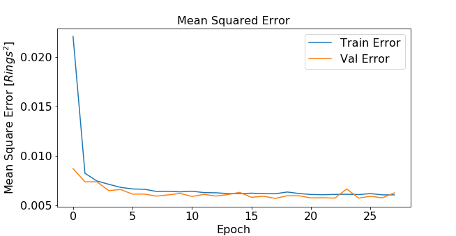
Error as function of epochs
Step 3: Prediction and Assessment of Model
Once our model is trained, we can use it to predict the age of the abalone in the test set. Once the values are predicted, then they must be re-scaled back which is performed using the inverse_transform function from Scikit-learn.
#Predict testing labels

y_pred= model.predict(X_test)

#undo normalization

y_pred_transformed=scalar.inverse_transform(y_pred.reshape(-1,1))
y_test_transformed=scalar.inverse_transform(y_test)
Then the predicted and actual ages are plotted along with a 1-to-1 line to visualize the performance of the model. An R-squared value and a RMSE are calculated as 0.554 and 2.20 rings respectively.
#visualize performance
fig, ax = plt.subplots()
ax.scatter(y_test_transformed, y_pred_transformed)
ax.plot([y_test_transformed.min(), y_test_transformed.max()], [y_test_transformed.min(), y_test_transformed.max()], 'k--', lw=4)
ax.set_xlabel('Measured (Rings)')
ax.set_ylabel('Predicted (Rings)')
plt.show()

#Calculate RMSE and R^2
from sklearn.metrics import mean_squared_error
from math import sqrt
rms = sqrt(mean_squared_error(y_test_transformed, y_pred_transformed))

from sklearn.metrics import r2_score
r_squared=r2_score(y_test_transformed,y_pred_transformed)

Predicted vs. Actual (Measured) Ages
The performance is not ideal, but the results are appropriate given that this dataset is notoriously hard to use for prediction without other relevant information such as weather or location. Ultimately, it is up to the user to decide if these are significant/acceptable values, otherwise the neural network hyperparameters can be further fine-tuned or more input data and more features can be added to the dataset to try to improve performance.
Sources:
[1]Dean, Jeff; Monga, Rajat; et al. (November 9, 2015). “TensorFlow: Large-scale machine learning on heterogeneous systems” (PDF). TensorFlow.org. Google Research.
[2] Yegulalp, Serdar. “What Is TensorFlow? The Machine Learning Library Explained.” InfoWorld, InfoWorld, 18 June 2019, http://www.infoworld.com/article/3278008/what-is-tensorflow-the-machine-learning-library-explained.html.
[3]“Keras: The Python Deep Learning Library.” Home – Keras Documentation, keras.io/.
[4] “Basic Regression: Predict Fuel Efficiency : TensorFlow Core.” TensorFlow, http://www.tensorflow.org/tutorials/keras/regression.


