On Parallelization of the Borg MOEA

This post will introduce basic concepts regarding the parallelization of the Borg Multiobjective Evolutionary Algorithm (Borg MOEA). In this post I’ll assume the reader is familiar with the basic architecture of the Borg MOEA, if you’re unfamiliar with the algorithm or would like a refresher, see Hadka and Reed, (2013a) before reading further.

Parallelization Basics

Before we go into parallization of Borg, let’s quickly define some terminology. Modern High Performance Computing (HPC) resources are usually comprised of many multi-core processors, each consisting of two or more processing cores. For this post, I’ll refer to an individual processing core as a “processor”. Parallel computing refers to programs that utilize multiple processors to simultaneously perform operations that would otherwise be performed in serial on a single processor.

Parallel computing can be accomplished using either “distributed” or “shared” memory methods. Shared memory methods consist of parallelizing tasks across a group of processors that all read and write from the same memory space. In distributed memory parallelization, each processor maintains its own private memory and data is usually passed between processors using a message passing interface (MPI) library. Parallel Borg applications are coded using distributed memory parallelization, though it’s important to note that it’s possible to parallelize the simulation model that is coupled with Borg using shared memory parallelization. For additional reading on parallelization concepts see Bernardo’s post from April and Barney’s posts from 2017.

Hadka et al., (2012) showed that the quality of search results discovered by the Borg MOEA is strongly dependent on the number of function evaluations (NFE) performed in an optimization run. Efficient parallelization of search on HPC resources can allow not only for the search to be performed “faster” but also may allow more NFE to be run, potentially improving the quality of the final approximation of the Pareto front. Parallelization also offers opportunities to improve the search dynamics of the MOEA, improving the reliability and efficiency of multi-objective search (Hadka and Reed, 2015; Salazar et al., 2017).

Below I’ll discuss two parallel implementations of the Borg MOEA, a simple master-worker implementation to parallelize function evaluations across multiple processors and an advanced hybrid multi-population implementation that improves search dynamics and is scalable Petascale HPC resources.

Master-worker Borg

Figure 1: The Master Worker implementation of the Borg MOEA. (Figure from Salazar et al., 2017)

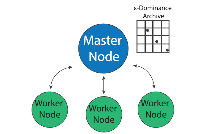
MOEA search is “embarrassingly parallel” since the evaluation of each candidate solution can be done independently of other solutions in a population (Cantu-Paz, 2000). The master-worker paradigm of MOEA parallelization, which has been in use since early days of evolutionary algorithms (Grefenstette, 1981), utilizes this property to parallelize search. In the master worker implementation of Borg in a system of P processors, one processor is designated as the “master” and P-1 processors are designated as “workers”. The master processor runs the serial version of the Borg MOEA but instead of evaluating candidate solution, it sends the decision variables to an available worker which evaluates the problem with the given decision variables and sends the evaluated objectives and constraints back to the master processor.

Most MOEAs are generational, meaning that they evolve a population in distinct stages known as generations (Coello Coello et al., 2007). During one generation, the algorithm evolves the population to produce offspring, evaluates the offspring and then adds them back into the population (methods for replacement of existing members vary according to the MOEA). When run in parallel, generational MOEAs must evaluate every solution in a generation before beginning evaluation of the next generation. Since these algorithms need to synchronize function evaluations within a generation, they are known as synchronous MOEAs. Figure 2, from Hadka et al., (2013b), shows a timeline of events for a typical synchronous MOEA. Algorithmic time (TA) represents the time it takes the master processor to perform the serial components of the MOEA. Function evaluation time (TF) is the the time it takes to evaluate one offspring and communication time (TC) is the time it takes to pass information to and from worker nodes. The vertical dotted lines in Figure 2 represent the start of each new generation. Note the periods of idle time that each worker node experiences while it waits for the algorithm to perform serial calculations and communicate. If the function evaluation time is not constant across all nodes, this idle time can increase as the algorithm waits for all solutions in the generation to be evaluated.

Figure 2: Diagram of a synchronous MOEA. Tc represents communication time, TA represents algorithmic time and TF represents function evaluation time. (Figure from Hadka et al., 2013b).

The Borg MOEA is not generational but rather a steady-state algorithm. As soon as an offspring is evaluated by a worker and returned to the master, the next offspring is immediately sent to the worker for evaluation. This is accomplished through use of a queue, for details of Borg’s queuing process see Hadka and Reed, (2015). Since Borg is not bound by the need to synchronize function evaluations within generations, it is known as an asynchronous MOEA. Figure 3, from Hadka et al., (2013b), shows a timeline of a events for a typical Borg run. Note that the idle time has been shifted from the workers to the master processor. When the algorithm is parallelized across a large number of cores, the decreased idle time for each worker has the potential to greatly increase the algorithm’s parallel efficiency. Furthermore, if function evaluation times are heterogeneous, the algorithm is not bottlenecked by slow evaluations as generational MOEAs are.

Figure 3: Diagram of an asynchronous MOEA. Tc represents communication time, TA represents algorithmic time and TF represents function evaluation time. (Figure from Hadka et al., 2013b).

While the master-worker implementation of the Borg MOEA is an efficient means of parallelizing function evaluations, the search algorithm’s search dynamics remain the same as the serial version and as the number of processors increases, the search may suffer from communication bottlenecks. The multi-master implementation of the Borg MOEA uses parallelization to not only improve the efficiency of function evaluations but also improve the quality of the multi-objective search.

Multi-Master Borg

Figure 4: The multi-master implementation of the Borg MOEA. (Figure from Salazar et al., 2017)

In population genetics, the “island model” considers distinct populations that evolve independently but periodically interbreed via migration events that occur over the course of the evolutionary process (Cantu-Paz, 2000). Two independent populations may evolve very different survival strategies based on the conditions of their environment (i.e. locally optimal strategies). Offspring of migration events that combine two distinct populations have the potential to combine the strengths developed by both groups. This concept has been utilized in the development of multi-population evolutionary algorithms (also called multi-deme algorithms in literature) that evolve multiple populations in parallel and occasionally exchange individuals via migration events (Cantu-Paz, 2000). Since MOEAs are inherently stochastic algorithms that are influenced by their initial populations, evolving multiple populations in parallel has the potential to improve the efficiency, quality and reliability of search results (Hadka and Reed, 2015; Salazar et al., 2017). Hybrid parallelization schemes that utilize multiple versions of master-worker MOEAs may further improve the efficiency of multi-population search (Cantu-Paz, 2000). However, the use of a multi-population MOEA requires the specification of parameters such as the number of islands, number of processors per island and migration policy that whose ideal values are not apparent prior to search.

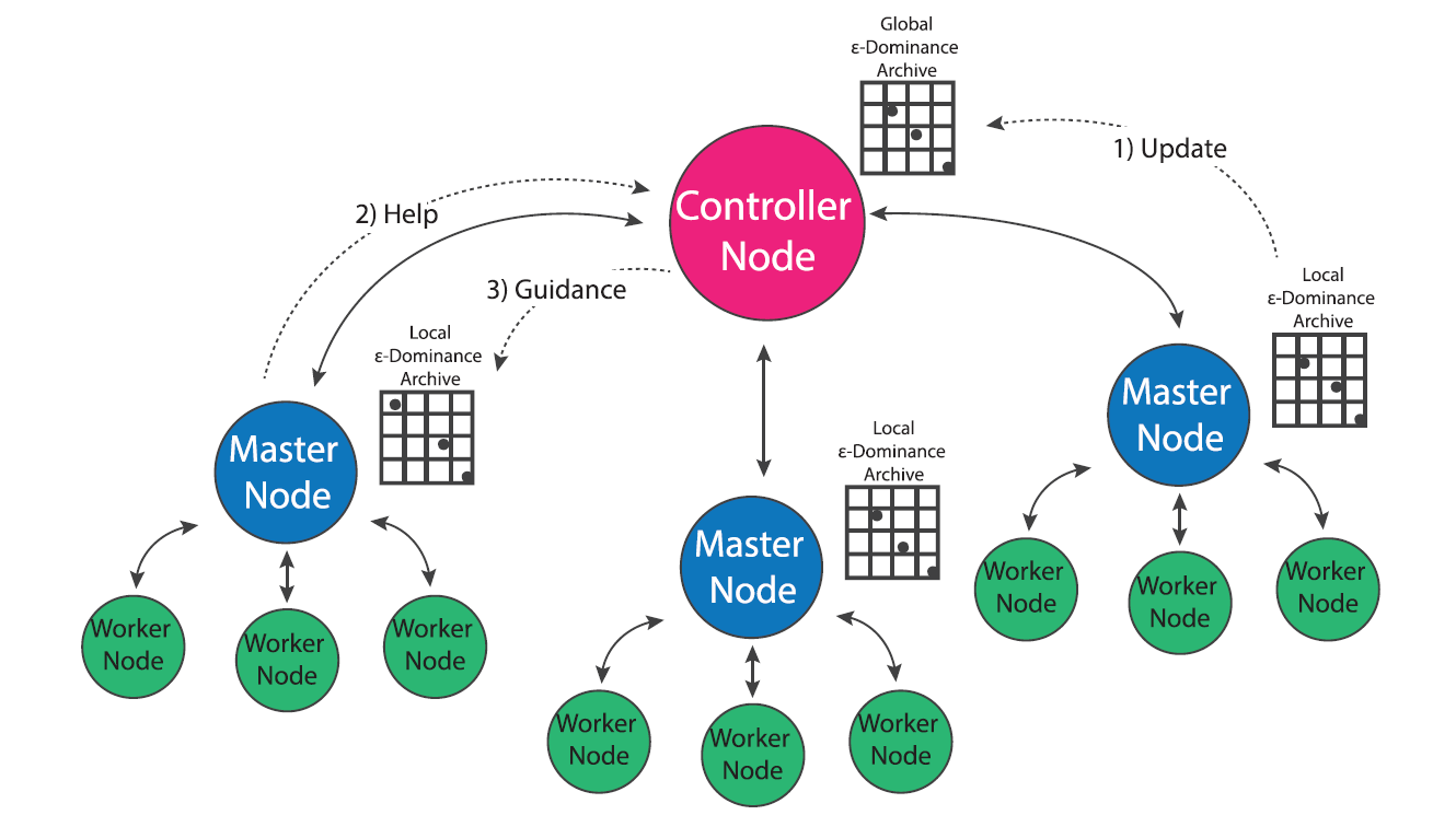
The multi-master implementation of the Borg MOEA is a hybrid parallelization of the MOEA that seeks to generalize the algorithm’s ease of use and auto-adaptivity while maximizing its parallel efficiency on HPC architectures (Hadka and Reed, 2015). In the multi-master implementation, multiple versions of the master-worker MOEA are run in parallel, and an additional processor is designated as the “controller”. Each master maintains its own epsilon dominance archive and operator probabilities, but regulatory updates its progress with the controller which maintains a global epsilon dominance archive and global operator probabilities. If a master processor detects search stagnation that it is not able to overcome via Borg’s automatic restarts, it requests guidance from the controller node which seeds the master with the contents of the global epsilon dominance archive and operator probabilities. This guidance system insures that migration events between populations only occurs when one population is struggling and only consists of globally non-dominated solutions. Borg’s adaptive population sizing ensures the injected population is resized appropriately given the global search state.

The use of multiple-populations presents an opportunity for the algorithm to improve the sampling of the initial population. The serial and master-worker implementations of Borg generate the initial population by sampling decision variables uniformly at random from their bounds, which has the potential to introduce random bias into the initial search population (Hadka and Reed, 2015). In the multi-master implementation of Borg, the controller node first generates a latin hypercube sample of the decision variables, then distributes these samples between masters uniformly at random. This initial sampling strategy adds some additional overhead to the algorithm’s startup, but ensures that globally the algorithm starts with a well-distributed, diverse set of initial solutions which can help avoid preconvergence (Hadka and Reed, 2015).

Conclusion

This post has reviewed two parallel implementations of the Borg MOEA. The next post in this series will discuss how to evaluate parallel performance of a MOEA in terms of search efficiency, quality and reliability. I’ll review recent literature comparing performance of master-worker and multi-master Borg and discuss how to determine which implementation is appropriate for a given problem.

References

Cantu-Paz, E. (2000). Efficient and accurate parallel genetic algorithms (Vol. 1). Springer Science & Business Media.

Hadka, D., Reed, P. M., & Simpson, T. W. (2012). Diagnostic assessment of the Borg MOEA for many-objective product family design problems. 2012 IEEE Congress on Evolutionary Computation (pp. 1-10). IEEE.

Hadka, D., & Reed, P. (2013a). Borg: An auto-adaptive many-objective evolutionary computing framework. Evolutionary computation, 21(2), 231-259.

Hadka, D., Madduri, K., & Reed, P. (2013b). Scalability analysis of the asynchronous, master-slave borg multiobjective evolutionary algorithm. In 2013 IEEE International Symposium on Parallel & Distributed Processing, Workshops and Phd Forum (pp. 425-434). IEEE.

Hadka, D., & Reed, P. (2015). Large-scale parallelization of the Borg multiobjective evolutionary algorithm to enhance the management of complex environmental systems. Environmental Modelling & Software, 69, 353-369.

Salazar, J. Z., Reed, P. M., Quinn, J. D., Giuliani, M., & Castelletti, A. (2017). Balancing exploration, uncertainty and computational demands in many objective reservoir optimization. Advances in water resources, 109, 196-210.

Introduction to Variable Infiltration Capacity (VIC) Model

The first time I read about the VIC model, I thought it was very complicated and was glad that I didn’t have to deal with it. Today, almost a decade later (which is scary for a different reason), I can say that I’m happy that this model has been a big part of my research life. I (and a lot of wonderful people, including my Ph.D. advisor Dr. Jennifer Adam) spent a lot of time coupling VIC to a cropping system model. The result is called VIC-CropSyst. We have been using this coupled model to answer questions about how the water system and agricultural systems interact. More on this later.

In this blog post, I provide some theoretical background to the variable infiltration capacity model, also known as the VIC model. In a future post, I’ll provide some hands-on exercises, but the main purpose of the present post is to provide some general, high-level intuitions for first-time users. With a lot of caution, I’ll add, many of these descriptions are valid for some other hydrological and land-surface models.

First, VIC is a land-surface hydrological model (Hamman et al., 2018; Liang et al., 1994). What this means is that it simulates different components of water and energy balance over land-surface areas. These components include runoff generation, base flow generation, water movement in soil, evaporation, transpiration components, and cold-season processes.

VIC is a deterministic, process-based model, meaning that it uses theoretically or statistically derived relationships to simulate water- and energy-system components. Keep in mind that this doesn’t mean that all these underlying relationships are correct. Many of them have been developed in specific circumstances and might not hold in others, and many of them use simplifying assumptions to make complicated physical relationships usable. This could be an interesting topic for another post.

VIC is a large-scale model. It has been used for basin-wide, regional, continental and global simulation of hydrological processes. The grid-cell resolution is an arbitrary number, but I have seen simulations using resolutions from 1/16 of a degree to 2 degrees.

VIC also captures some key inter-grid cell variabilities. This means that when VIC simulates a grid cell, it divides the cells into subsections and simulates the hydrological processes for each of those. This is important because, as I mentioned, VIC is a large-scale model, and there might be a lot of variability within (let’s say) a 12 × 12 km grid cell. We might have lakes, mountains, valleys, forests, and agricultural land. VIC takes the original meteorological data and laps to different elevation levels of a grid cell (called snow bands in VIC).

VIC is also a spatially distributed model. This means that if you’re interested in running the model over a large basin, you need to divide the area into several grid cells with the same resolution. Then you run the model over each individual cell. The model’s time steps can range from hourly to daily.

In terms of time and space continuums, VIC has two main modes: (1) space before time, and (2) time before space. Each method comes with some computational pros and cons and some specific reasons. Space before time. In each time step, the model goes to one individual grid cell, runs for one time step, and then moves on to the next cell. When all the cells have been done for that time step, the model goes to the next time step and the process continues. Version 5 of VIC has the capability to simulate this, and this mode of the model is called image mode.

Time before space. The model starts the simulation with one grid cell, finishes it for all the time steps, and then moves on to the next cell. All versions of VIC can carry out time-before-space simulations .

Some More Technical Details

Variable infiltration capacity curve. As might be obvious from the name, this curve is one of the most important underlying processes in the model. A crucial part of each hydrological model is the partitioning of rainfall into runoff and infiltration. The basic idea came from a study of the spatial relations between runoff generation and soil moisture in large river basins (Xianjiang model; Zhao et al., 1980): when soil moisture is higher, more water goes into runoff, and when soil moisture is lower, infiltration is higher. The model uses these curves to partition precipitation into runoff and infiltration. The main parameter of the variable infiltration capacity curve (bi) is treated as a calibration parameter. Here is the VIC curve formula:

Movement of water in soil. VIC usually has three main soil layers. Once water enters the soil, it is distributed vertically from the top to the bottom layer. The top layer is usually 10 cm, which ensures that the calculation of evaporation from the soil is reasonable (see Liang et al., (1996)). The middle layer usually takes care of conveying the water to the next soil layer; it also acts as a reservoir of water for the crop root zone. The last layer is called the base flow layer. Once water reaches this layer, it stays there until it goes out of the system as base flow. The following figure shows a very simplified schematic of VIC soil layering system and sum of the key processes discussed here.

Base flow. VIC uses a two-stage base flow curve developed by Franchini and Pacciani, (1991). The first stage is linear. Basically, when the soil moisture is below a certain limit, the base flow generation has a linear relationship with soil moisture in the bottom layer of VIC (i.e., more moisture leads to more base flow). After that threshold, base flow generation increases exponentially with soil moisture until the soil moisture drops below that linearity limit. There are a few important calibration parameters in the formulation of base flow.

Energy balance. In each time step, VIC simulates many components of land-surface energy-related processes, such as snow accumulation and thawing, frozen soil and permafrost processes, evapotranspiration, and canopy-level energy budget (Cherkauer and Lettenmaier, 1999). Obviously, the different components of the energy balance are in continuous interaction with the water-balance components.

Model Inputs

At minimum, VIC needs the following information as inputs to the model: (1) meteorological data (e.g., minimum and maximum temperature, precipitation, and wind speed), (2) soil-texture information (e.g., hydraulic conductivity, initial moisture, moisture at field capacity, and permanent wilting point), and (3) land-use data (e.g., bare soil, open water, vegetation, depth of roots of the vegetation cover). However, the complete list of input parameters is much longer. I will go through these details in the next post.

Model Output

Some of the model’s fluxes and states are distributed by nature, such as evaporation, transpiration, and soil moisture. Others are aggregated, of which the most important is stream flow. To calculate stream flow, another step is needed to calculate runoff. VIC then aggregates the runoff and base flow generated from each individual grid cell to the outlet of basin. This process happens outside the main body of VIC (as a post-processing step) and is called routing (Lohmann et al., 1998). There are many other outputs users can choose at the end of simulation. For a complete list, look at this webpage.

To recap, the main focus of this is the VIC model. As I mentioned, however, VIC-CropSyst is a coupled version of VIC model, and in this version a process-based agricultural model is used to simulate agricultural processes such as crop growth, transpiration, root and shoot development, canopy coverage, and responses to climatic stressors. I haven’t covered it in this post, but maybe I’ll go back to it in a few months. In the meantime, for more information you can refer to (Malek et al., 2018, 2017).

References

Cherkauer, K.A., Lettenmaier, D.P., 1999. Hydrologic effects of frozen soils in the upper Mississippi River basin. J. Geophys. Res. Atmospheres 104, 19599–19610. https://doi.org/10.1029/1999JD900337

Franchini, M., Pacciani, M., 1991. Comparative analysis of several conceptual rainfall-runoff models. J. Hydrol. 122, 161–219. https://doi.org/10.1016/0022-1694(91)90178-K

Hamman, J.J. (ORCID:0000000174798439), Nijssen, B. (ORCID:0000000240620322), Bohn, T.J., Gergel, D.R., Mao, Y., 2018. The Variable Infiltration Capacity model version 5 (VIC-5): infrastructure improvements for new applications and reproducibility. Geosci. Model Dev. Online 11. https://doi.org/10.5194/gmd-11-3481-2018

Liang, X., Lettenmaier, D.P., Wood, E.F., Burges, S.J., 1994. A simple hydrologically based model of land surface water and energy fluxes for general circulation models. J. Geophys. Res. Atmospheres 99, 14415–14428. https://doi.org/10.1029/94JD00483

Liang, X., Wood, E.F., Lettenmaier, D.P., 1996. Surface soil moisture parameterization of the VIC-2L model: Evaluation and modification. Glob. Planet. Change 13, 195–206. https://doi.org/10.1016/0921-8181(95)00046-1

LOHMANN, D., RASCHKE, E., NIJSSEN, B., LETTENMAIER, D.P., 1998. Regional scale hydrology: I. Formulation of the VIC-2L model coupled to a routing model. Hydrol. Sci. J. 43, 131–141. https://doi.org/10.1080/02626669809492107

Malek, K., Adam, J.C., Stöckle, C.O., Peters, R.T., 2018. Climate change reduces water availability for agriculture by decreasing non-evaporative irrigation losses. J. Hydrol. 561, 444–460. https://doi.org/10.1016/j.jhydrol.2017.11.046

Malek, K., Stöckle, C., Chinnayakanahalli, K., Nelson, R., Liu, M., Rajagopalan, K., Barik, M., Adam, J.C., 2017. VIC–CropSyst-v2: A regional-scale modeling platform  to simulate the nexus of climate, hydrology, cropping  systems, and human decisions. Geosci Model Dev 10, 3059–3084. https://doi.org/10.5194/gmd-10-3059-2017

Zhao, R.J., Zhang, Y.L., Fang, L.R., others, 1980. The Xinanjiang model Hydrological Forecasting Proceedings Oxford Symposium. Oxford: IASH.

Packages for Hydrological Data Retrieval and Statistical Analysis

I recently searched for publicly available code to run statistical analyses that are commonly employed to evaluate (eco)hydrology datasets. My interests included data retrieval, data visualization, outlier detection, and regressions applied to streamflow, water quality, weather/climate, and land use data. This post serves as a time snapshot of available code resources.

Package Languages

I focused on packages in R and Python. R seems to have more data analysis and statistical modeling packages, whereas Python seems to have more physical hydrological modeling packages. As a result of my search interests, this post highlights the available R packages. Here are good package lists for both languages:

• R Hydrology Package List
• Python Hydrology Package List

Hopefully, the time required to prepare your data and learn how to use these functions is less than the time to develop similar functions yourself. Most packages have vignettes (tutorials) that should help to learn the functions, and may also serve as teaching resources. In R, the function browseVignettes(‘packageName’) will open a webpage containing links to vignette PDFs (if available) and source code resources for the specified package. The datasets.load package in R is useful to discover if a specified package has sample datasets available to use.

Example webpage output from browseVignettes(‘smwrQW’):

Webpage link

USGS R Packages

R is currently the primary development language for hydrological statistical analyses within the United States Geological Survey (USGS). There are nearly 100 USGS-R Github repositories, from which I’ve selected a subset that seem to be actively maintained and applicable to the interests listed above. I’m not sure if similar functions as the ones contained within these repositories are available and tested in other programming languages. These USGS-R packages have test functions, which provides a baseline level of confidence in their development. Many packages are contributed or maintained by Laura DeCicco, and by David Lorenz for statistical analysis and water quality.

• USGS R Package Documentation Site
• USGS R Github Repositories

Selected USGS R Packages

• dataRetrieval for streamflow and water quality gauge/site data retrieval from the National Water Information System (NWIS) and the Water Quality Portal (WQP). This package has several great vignettes that demonstrate how to use the functions. The package is simple to use, but the data require processing to be useful for research (I’m currently developing a code repository for this purpose).
• Statistical Methods in Water Resources (smwr). All have vignettes.

smwrBase: Generic hydrology data processing tools

smwrStats: Statistical analysis and probability functions, and a possible companion book by Helsel and Hirsch (2002)

• WREG: Predictions in ungauged basins w/ OLS, GLS, WLS
• nsRFA: Regional Frequency Analysis, focusing on the index-value method
• DVstats: Daily flow statistical analysis and visualization
• HydroTools: Seems useful based on the function names, but no documentation outside of the functions themselves. Seems to be under development.

 

Additional R Hydrology Packages

• hydroTSM: Excellent graphics package for time series data. Two examples below of one-line plot functions and summary statistics.
  

  
• fasstr: hydrological time series analysis with a quick-start Cheat Sheet
• FlowScreen: temporal trends and changepoint analysis
• hydrostats: Computation of daily streamflow metrics (e.g. low flows, high flows, seasonality)
• FAdist: Common probability distributions for frequency analysis. These distributions are not available in base R.
• lmom and lmomRFA: L-moments for common probability distributions, and regional frequency analysis.
• nhdR: National Hydrography Dataset downloads

 

Water Quality

• EGRET – Excellent for plotting water quality data
  User guide
  Confidence intervals for WRTDS regression method
• smwrQW: USGS water quality data processing. Seems better than EGRET for quantitative water quality data analysis functions.

 

Streamflow & Weather Generators

• MATLAB Kirsch-Nowak Streamflow Generator and blog posts
• RMAWGEN: Multi-site Auto-regressive Weather GENerator in R
• weathergen: for synthetic climate timeseries

 

Weather Station Data

• rnoaa: NOAA station data downloads using R (tip: the meteo_tidy_ghcnd() function provides nicely formated year-month-day datasets)
  • GHCNpy: similar package in Python for GHCN-Daily records. Also has visualization functions.
• countyweather: US County-level weather data
• getMet: Seems like a SWAT model companion for weather data
• meteo: Data Analysis and Visualization

 

Climate Assessment

• musica: Climate model assessment tools

 

Hydrological Models in R:

• topmodel: Topmodel for flow modeling
• swmmr: SWMM model for stormwater
• swatmodel: SWAT model for ecohydrological studies

 

Land Use / Land Cover Change

• lulcc: Land Use and Land Cover Change modeling

 

If you know of other good packages, please add them to the comments or write to me so that I can add them to the lists.

MOEAFramework Training Part 3: Calculating Metrics

Part 3 of the MOEAFramework Training covers calculation of metrics that can be used to assess the performance of your algorithms. The relevant files and folders for this part of the training have been added to the Github repo. These are:

• generate_refset.sh
• evaluate.sh 

Generation of a Reference Set

In order to assess the performance of an algorithm, you have to have something to compare its approximation sets to. If your optimization problem has a theoretical solution, then the approximation sets produced by the run.sh script in Part 2 can be compared against a theoretical reference set. However, most real world optimization problems do not have a solution. Therefore, a best known reference set must be used for comparison. The best known reference set is usually generated by combining the best solutions from all algorithms that are tested.

generate_refset.sh uses MOEAFramework’s ResultFileMerger class to first merge all seeds of one parameterization into a merged set (i.e. NSGAII_lake_P2.set). Then, the script implements the ReferenceSetMerger class to combine all parameterizations into one overall algorithm reference set (i.e. Borg_lake.set) based on the epsilons provided in the settings.sh script. Finally, the ReferenceSetMerger is once again used to determine an overall best reference set across all algorithms (i.e. lake.ref). After running ./generate_refset.sh, the corresponding files will be stored in the folder data_ref. At this point, one can then make a 3D plot of the overall reference set and the algorithm-specific reference sets to start visualizing differences in algorithms. The figure below shows the best-known reference set for the DPS version of the lake problem found by plotting the solutions in lake.ref as well as the best reference sets for Borg and NSGA-II found after running 10 seeds and 10 parameterizations of the algorithms for 25,000 NFE. For a more thorough diagnostic experiment, usually 20-50 seeds of 100 parameterizations of each algorithm are run for around 100,000 NFE.

Calculation of Performance Metrics

From the figures, differences in each algorithm’s reference set can be seen. Notably, Borg is able to produce solutions with a much higher reliability than NSGA-II and ultimately it seems as though mostly Borg’s solutions contribute to the overall reference set. Depending on the complexity of the problem, these differences will become more apparent. To more formally quantify algorithm performance, we use the ResultFileEvaluator in the evaluate.sh script to calculate performance metrics including hypervolume, generational distance, and epsilon indicator using the raw optimization results and the overall reference set. More information on these metrics and how to calculate them can be found in Evolutionary Algorithms for Solving Multi-Objective Problems by Coello Coello (2007). Note that the metrics are reported every 100 NFE, as defined in the run.sh file. After running ./evaluate.sh, metric files will be stored in the data_metrics folder. A metric file will be created for each seed of each parameterization. Ultimately, as will be shown in the next post, these files can be averaged across seeds and/or parameterizations to determine average performance of an algorithm.

In the next post, we will show how to merge these metrics and effectively visualize them to assess the performance of the algorithm over time and over different parameterizations.