Introduction To Econometrics: Part II- Violations of OLS Assumptions & Methods for Fixing them

Regression is the primary tool used in econometrics to infer relationships between a group of explanatory variables, X and a dependent variable, y. My previous post focused on the mechanics of Ordinary Least Squares (OLS) Regression and outlined key assumptions that, if true, make OLS estimates the Best Linear Unbiased Estimator (BLUE) for the coefficients in the regression:

This post will discuss three common violations of OLS assumptions, and explain tools that have been developed for dealing with these violations. We’ll start with a violation of the assumption of a linear relationship between X and y, then discuss heteroskedasticity in the error terms and the issue of endogeniety.

Linearity

If the relationship between X and y is not linear, OLS can no longer be used to estimate beta. A nonlinear regression of y on X has the form:

Where  g(X\beta) is the functional form of the nonlinear relationship between X and y and epsilon is the error term. Beta can be estimated using Nonlinear Least Squares regression (NLS). Similar  to OLS regression, NLS seeks to minimize the sum of the square error term.

To solve for beta, we again take the derivative and set it equal to zero, but for the nonlinear system there is no closed form solution, so the estimators have to be found using numerical optimization techniques.

The variance of a NLS estimator is:

Where G is a matrix of partial derivatives of g with respect to each Beta.

Modern numerical optimization techniques can solve many NLS equations quite easily making NLS a common alternative to OLS regression especially when there is a hypothesized functional form for the relationship between X and y.

Heteroskedasticity

Heteroskedasticity arises within a data set when the errors do not have a constant variance with respect to X. In equation form, under heteroskedasticity:

The presence of heteroskedasticity  increases the variance of Beta estimators found using OLS regression, reducing the efficiency of the estimator and causing it to no longer be the BLUE. As put by Allison (2012), OLS on heteroskedastic data puts “equal weight on all observations when, in fact, observations with larger disturbances contain less information”.

To fix this problem, econometric literature provides two options which both use a form of weighting to correct for differences in variance amongst the error terms:

1. Use the OLS estimate for beta, but calculate the variance of beta with a robust variance-covariance matrix .
2. Estimate Beta using Feasible Generalized Least Squares (FGLS)

Let’s begin with the first strategy, using OLS beta estimates with a robust variance-covariance matrix. The robust variance-covariance matrix can be derived using the Generalized Method of Moments (GMM) for the sake of brevity, I’ll omit the derivation here and skip to the final result:

Where is a matrix of square residuals from the OLS regression:

The second strategy, estimation using FGLS, requires a more involved process for estimating beta. FGLS can be accomplished through 3 steps:

1. Use OLS to find OLS estimate for beta and calculate the residuals:

2. Regress the error term on a subset of X, which we will call Z, to get an estimate of a new parameter, theta (denoted with a tilde, but wordpress makes it difficult for me to add this in the middle of a paragraph). We then use this parameter to estimate the variance of the error term, sigma squared,  for each observation:

A diagonal matrix, D (different than the D used for the robust variance-covariance matrix), is then constructed using these variance estimates.

3. Finally, we use the matrix D to find our FGLS estimator for beta:

The variance of of the FGLS beta etimate is then defined as:

Endogeneity

Endogeneity arises when explanatory variables are correlated with the error term in a regression. This may be a result of simultaneity, when errors and explanatory variables are effected by the same exogenous influences, omitted variable bias,  when an important variable is left out of a regression, causing the over- or underestimation of the effect of other explanatory variables and the error term, measurement error or a lag in the dependent variable. Endogeniety can be hard to detect and may cause regression large errors in regression results.

A common way of correcting for endogeniety is through Instrumental Variables (IVs). Instrumental variables are explanatory variables that are highly correlated with variables that cause endogeniety but are exogenous to the system. Examples include using proximity to cardiac care centers as an IV for heart surgery when modeling health or state cigarette taxes as an IV for maternal smoking rate when modeling infant birth weight (Angrist and Kruger, 2001). For an expansive but accessible overview of IVs and their many applications, see Angrist and Kruger (2001).

A common technique for conducting a regression using IVs is 2 Stage Least Squares (2SLS) regression. The two stages of 2SLS are as follows:

1. Define Z as a new set of explanatory variables, which omits the endogenous variables and includes the IVs (which are usually not included in the original OLS regression).
2. Project Z onto the column space of X.
3. Estimate the 2SLS using this projection:

Using 2SLS regression to correct for endogeneity is fairly simple, however identifying good IVs for an endogenous variable can be extremely difficult. Finding a good IV (or set of IVs) can be enough to get one published in an economics journal (at least that’s what my economist friend told me).

Concluding thoughts

These two posts have constituted an extremely brief introduction to the field of econometrics meant for engineers who may be interested in learning about common empirical tools employed by economists. We covered the above methods in much more detail in class and also covered other topics such as panel data, Generalize Method Of Moments estimation, Maximum Likelihood Estimation, systems of equations in regression and discrete choice modeling. Overall, I found the course (AEM 7100) to be a useful introduction to a field that I hope to learn more about over the course of my PhD.

References:

Allison, Paul D. (2012). “Multiple regression: a primer“. Pine Forge. Thousand Oaks, CA: Press Print.

Angrist, J.; Krueger, A. (2001). “Instrumental Variables and the Search for Identification: From Supply and Demand to Natural Experiments”. Journal of Economic Perspectives. 15 (4): 69–85. doi:10.1257/jep.15.4.69.

An Introduction To Econometrics: Part 1- Ordinary Least Squares Regression

I took a PhD level econometrics course this semester in the Applied Economics and Management department here at Cornell and I thought I’d share some of what I learned. Overall, I enjoyed the course and learned a great deal. It was very math and theory heavy, but the Professor Shanjun Li did a nice job keeping the class lively and interesting. I would recommend the class to future EWRS students who may be looking for some grounding in econometrics, provided they’ve taken some basic statics and linear algebra courses.

So lets start with the basics, what does the term “econometrics” even mean? Hansen (2010) defined econometrics as “the unified study of economic models, mathematical statistics and economic data”. After taking this introductory course, I’m inclined to add my own definition: econometrics is “a study of the problems with regression using Ordinary Least Squares (OLS) and how to solve them”. This is obviously a gross oversimplification of the field, however, regression through OLS was the primary tool used for finding insights and patterns within data, and we spent the vast majority of the course examining it. In this post I’ll briefly summarize OLS mechanics and classical OLS assumptions. In my next post, I’ll detail methods for dealing with violations of OLS assumptions. My hope is that reading this may help you understand some key terminology and the reasoning behind why certain econometric tools are employed.

OLS mechanics

Our primary interest when creating an econometric model is to estimate some dependent variable, y, using a observations from a set of independent variables, X. Usually y is a vector of length n, where n is the number of observations, and X is a matrix of size (n x k) where k is the number of explanatory variables (you can think of X as a table of observations, where each column contains a different variable and each row represents an observation of that variable). The goal of OLS regression is to estimate the coefficients, beta, for the model:

Where beta is a k by 1 vector of coefficients on X and epsilon is a k by 1 vector of error terms.

OLS regression estimates beta by minimizing the sum of the square error term (hence the name “least squares”). Put in matrix notation, OLS estimates beta using the equation:

The optimal beta estimate can be found through the following equations:

Taking the derivative and setting it equal to zero:

Then solving for the beta estimate:

 

Estimation of y using OLS regression can be visualized as the orthogonal projection of the vector y onto the column space of X. The estimated error term, epsilon, is the orthogonal distance between the projection and the true vector y.  Figure 1 shows this projection for a y that is regressed on two explanatory variables, X1 and X2.

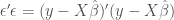
Figure 1: OLS regression as an orthogonal projection of vector y onto the column space of matrix X. The error term, , is the orthogonal distance between y and . (Image source: Wikipedia commons)

 Assumptions and properties of OLS regression

The Gauss-Markov Theorem states that under a certain set of assumptions, the OLS estimator is the Best Linear Unbiased Estimator (BLUE) for vector y.

To understand the full meaning of the Gauss-Markov theorem, it’s important to define two fundamental properties that can be used to describe estimators, consistency and efficiency. An estimator is consistent if its value will converge to the true parameter value as the number of observations goes to infinity. An estimator is efficient if its asymptotic variance is no larger than the asymptotic variance of any other possible consistent estimator for the parameter. In light of these definitions, the Gauss-Markov Theorem can be restated as: estimators found using OLS will be the most efficient consistent estimator for beta as long as the classical OLS assumptions hold. The remainder of this post will be devoted to describing the necessary assumptions for the OLS estimator to be the BLUE and detailing fixes for when these assumptions are violated.

The four classical assumptions for OLS to be the BLUE are:

1. Linearity: The relationship between X and y is linear, following the functional form:

.

2. Strict exogeneity: The error terms should be independent of the value of the explanatory variables, X. Put in equation form, this assumption requires:

3.  No perfect multicollinearity: columns of X should not be correlated with each other (see my earlier post on dealing with mulitcollinearity for fixes for violations of this assumption).

4. Spherical Error: Error terms should be homoskedastic, meaning they are evenly distributed around the X values. Put in equation form:

Where is a constant value.

Using assumption 4, we can define the variance of  as:

If assumptions 1-4 hold, then the OLS estimate for beta is the BLUE, if however, any of the assumptions are broken, we must employ other methods for estimating our regression coefficients.

In my next post I’ll detail the methods econometricians use when these assumptions are violated.

 References:

Hansen, Bruce. “Econometrics”. 2010. University of Wisconsin

Click to access Econometrics2010.pdf