Types of Errors in Numerical Methods

What are numerical methods?

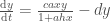
Many engineering problems are too time consuming to solve or may not be able to be solved analytically. In these situations, numerical methods are usually employed. Numerical methods are techniques designed to solve a problem using numerical approximations. An example of an application of numerical methods is trying to determine the velocity of a falling object. If you know the exact function that determines the position of your object, then you could potentially differentiate the function to obtain an expression for the velocity. More often, you will use a machine to record readings of times and positions that you can then use to numerically solve for velocity:

where f is your function, t is the time of the reading, and h is the distance to the next time step.

Because your answer is an approximation of the analytical solution, there is an inherent error between the approximated answer and the exact solution. Errors can result prior to computation in the form of measurement errors or assumptions in modeling. The focus of this blog post will be on understanding two types of errors that can occur during computation: roundoff errors and truncation errors.

Roundoff Error

Roundoff errors occur because computers have a limited ability to represent numbers. For example, π has infinite digits, but due to precision limitations, only 16 digits may be stored in MATLAB. While this roundoff error may seem insignificant, if your process involves multiple iterations that are dependent on one another, these small errors may accumulate over time and result in a significant deviation from the expected value. Furthermore, if a manipulation involves adding a large and small number, the effect of the smaller number may be lost if rounding is utilized. Thus, it is advised to sum numbers of similar magnitudes first so that smaller numbers are not “lost” in the calculation.

One interesting example that we covered in my Engineering Computation class, that can be used to illustrate this point, involves the quadratic formula. The quadratic formula is represented as follows:

Using a = 0.2, b = – 47.91, c = 6 and if we carry out rounding to two decimal places at every intermediate step:

The error between our approximations and true values can be found as follows:

As can be seen, the smaller root has a larger error associated with it because deviations will be more apparent with smaller numbers than larger numbers.

If you have the insight to see that your computation will involve operations with numbers of differing magnitudes, the equations can sometimes be cleverly manipulated to reduce roundoff error. In our example, if the quadratic formula equation is rationalized, the resulting absolute error is much smaller because fewer operations are required and numbers of similar magnitudes are being multiplied and added together:

Truncation Error

Truncation errors are introduced when exact mathematical formulas are represented by approximations. An effective way to understand truncation error is through a Taylor Series approximation. Let’s say that we want to approximate some function, f(x) at the point x_i+1, which is some distance, h, away from the basepoint x_i, whose true value is shown in black in Figure 1. The Taylor series approximation starts with a single zero order term and as additional terms are added to the series, the approximation begins to approach the true value. However, an infinite number of terms would be needed to reach this true value.

Figure 1: Graphical representation of a Taylor Series approximation (Chapra, 2017)

The Taylor Series can be written as follows:

where R_n is a remainder term used to account for all of the terms that were not included in the series and is therefore a representation of the truncation error. The remainder term is generally expressed as R_n=O(hⁿ⁺¹) which shows that truncation error is proportional to the step size, h, raised to the n+1 where n is the number of terms included in the expansion. It is clear that as the step size decreases, so does the truncation error.

The Tradeoff in Errors

The total error of an approximation is the summation of roundoff error and truncation error. As seen from the previous sections, truncation error decreases as step size decreases. However, when step size decreases, this usually results in the necessity for more precise computations which consequently results in an increase in roundoff error. Therefore, the errors are in direct conflict with one another: as we decrease one, the other increases.

However, the optimal step size to minimize error can be determined. Using an iterative method of trying different step sizes and recording the error between the approximation and the true value, the following graph shown in Figure 2 will result. The minimum of the curve corresponds to the minimum error achievable and corresponds to the optimal step size. Any error to the right of this point (larger step sizes) is primarily due to truncation error and the increase in error to the left of this point corresponds to where roundoff error begins to dominate. While this graph is specific to a certain function and type of approximation, the general rule and shape will still hold for other cases.

Figure 2: Plot of Error vs. Step Size (Chapra, 2017)

Hopefully this blog post was helpful to increase awareness of the types of errors that you may come across when using numerical methods! Internalize these golden rules to help avoid loss of significance:

• Avoid subtracting two nearly equal numbers
• If your equation has large and small numbers, work with smaller numbers first
• Consider rearranging your equation so that numbers of a similar magnitude are being used in an operation

Sources:

Chapra, Steven C. Applied Numerical Methods with MATLAB for Engineers and Scientists. McGraw-Hill, 2017.

Class Notes from ENGRD 3200: Engineering Computation taught by Professor Peter Diamessis at Cornell University

Plotting trajectories and direction fields for a system of ODEs in Python

The aim of this post is to guide the reader through plotting trajectories and direction fields for a system of equations in Python. This is useful when investigating the equilibria and stability of the system, and to facilitate in understanding the general behavior of a system under study. I will use a system of predator-prey equations, that my most devoted online readers are already familiar with from my previous posts on identifying equilibria and stability, and on nondimensionalization. Specifically, I’ll be using the Lotka-Volterra set of equations with Holling’s Type II functional response:

where:

x: prey abundance

y: predator abundance

b: prey growth rate

d: predator death rate

c: rate with which consumed prey is converted to predator

a: rate with which prey is killed by a predator per unit of time

K: prey carrying capacity given the prey’s environmental conditions

h: handling time

This system has 3 equilibria: when both species are dead (0,0), when predators are dead and the prey grows to its carrying capacity (K,0) and a non-trivial equilibrium where both species coexist and is generally more interesting, given by:

The following code should produce both trajectories and direction fields for this system of ODEs (python virtuosos please excuse the extensive commenting, I try to comment as much as possible for people new to python):

import numpy as np
from matplotlib import pyplot as plt
from scipy import integrate

# I'm using this style for a pretier plot, but it's not actually necessary
plt.style.use('ggplot')

"""
This is to ignore RuntimeWarning: invalid value encountered in true_divide
I know that when my populations are zero there's some division by zero and
the resulting error terminates my function, which I want to avoid in this case.
"""
np.seterr(divide='ignore', invalid='ignore')

# These are the parameter values we'll be using
a = 0.005
b = 0.5
c = 0.5
d = 0.1
h = 0.1
K = 2000

# Define the system of ODEs
# P[0] is prey, P[1] is predator
def fish(P, t=0):
    return ([b*P[0]*(1-P[0]/K) - (a*P[0]*P[1])/(1+a*h*P[0]),
            c*(a*P[0]*P[1])/(1+a*h*P[0]) - d*P[1] ])

# Define equilibrium point
EQ = ([d/(a*(c-d*h)),b*(1+a*h*(d/(a*(c-d*h))))*(1-(d/(a*(c-d*h)))/K)/a])

"""
I need to define the possible values my initial points will take as they
relate to the equilibrium point. In this case I chose to plot 10 trajectories
ranging from 0.1 to 5
"""
values = np.linspace(0.1, 5, 10)
# I want each trajectory to have a different color
vcolors = plt.cm.autumn_r(np.linspace(0.1, 1, len(values)))

# Open figure
f = plt.figure()
"""
I need to define a range of time over which to integrate the system of ODEs
The values don't really matter in this case because our system doesn't have t
on the right hand side of dx/dt and dy/dt, but it is a necessary input for
integrate.odeint.
"""
t = np.linspace(0, 150, 1000)

# Plot trajectories by looping through the possible values
for v, col in zip(values, vcolors):
    # Starting point of each trajectory
    P0 = [E*v for E in EQ]
    # Integrate system of ODEs to get x and y values
    P = integrate.odeint(fish, P0, t)
    # Plot each trajectory
    plt.plot( P[:,0], P[:,1],
            # Different line width for different trajectories (optional)
            lw=0.5*v,
            # Different color for each trajectory
            color=col,
            # Assign starting point to trajectory label
            label='P0=(%.f, %.f)' % ( P0[0], P0[1]) )
"""
To plot the direction fields we first need to define a grid in order to
compute the direction at each point
"""
# Get limits of trajectory plot
ymax = plt.ylim(ymin=0)[1]
xmax = plt.xlim(xmin=0)[1]
# Define number of points
nb_points = 20
# Define x and y ranges
x = np.linspace(0, xmax, nb_points)
y = np.linspace(0, ymax, nb_points)
# Create meshgrid
X1 , Y1 = np.meshgrid(x,y)
# Calculate growth rate at each grid point
DX1, DY1 = fish([X1, Y1])
# Direction at each grid point is the hypotenuse of the prey direction and the
# predator direction.
M = (np.hypot(DX1, DY1))
# This is to avoid any divisions when normalizing
M[ M == 0] = 1.
# Normalize the length of each arrow (optional)
DX1 /= M
DY1 /= M

plt.title('Trajectories and direction fields')
"""
This is using the quiver function to plot the field of arrows using DX1 and
DY1 for direction and M for speed
"""
Q = plt.quiver(X1, Y1, DX1, DY1, M, pivot='mid', cmap=plt.cm.plasma)
plt.xlabel('Prey abundance')
plt.ylabel('Predator abundance')
plt.legend(bbox_to_anchor=(1.05, 1.0))
plt.grid()
plt.xlim(0, xmax)
plt.ylim(0, ymax)
plt.show()

This should produce the following plot. All P0s are the initial conditions we defined.

We can also see that this parameter combination produces limit cycles in our system. If we change the parameter values to:

a = 0.005
b = 0.5
c = 0.5
d = 0.1
h = 0.1
K = 200

i.e. reduce the available resources to the prey, our trajectories look like this:

The equilibrium becomes stable, attracting the trajectories to it.

The same can be seen if we increase the predator death rate:

a = 0.005
b = 0.5
c = 0.5
d = 1.5
h = 0.1
K = 2000

The implication of this observation is that an initially stable system, can become unstable given more resources for the prey or less efficient predators. This has been referred to as the Paradox of Enrichment and other predator-prey models have tried to address it (more on this in future posts).

P.S: I would also like to link to this scipy tutorial, that I found very helpful and that contains more plotting tips.