MORDM Basics VI: Processing the output and reevaluating for robustness

In the previous post, we conducted a basic WaterPaths tutorial in which we ran a simulation-optimization of the North Carolina Research Triangle test case (Trindade et al, 2019); across 1000 possible futures, or states of the world (SOWs). To briefly recap, the Research Triangle test case consists of three water utilities in Cary (C), Durham (D) and Raleigh (R). Cary is the main supplier, having a water treatment plant of its own. Durham and Raleigh purchase water from Cary via treated transfers.

Having obtained the .set file containing the Pareto-optimal decision variables and their respective performance objective values, we will now walk through the .set file processing and visualize the decision variables and performance objective space.

Understanding the .set file

First, it is important that the .set file makes sense. The NC_output_MS_S3_N1000.set file should have between 30-80 rows, and a total of 35 columns. The first 20 columns contain values of the decision variables. Note that only Durham and Raleigh have water transfer triggers as they purchase treated water from Cary.

1. Restriction trigger, RT (C, D, R)
2. Transfer trigger, TT (D, R)
3. Jordan Lake allocation, JLA (C, D, R)
4. Reserve fund contribution as a percentage of total annual revenue, RC (C, D, R)
5. Insurance trigger, IT (C, D, R)
6. Insurance payments as a percentage of total annual revenue, IP (C, D, R)
7. Infrastructure trigger, INF (C, D, R)

The last 15 columns contain the objective values for the following performance objectives of all three utilities:

1. Reliability (REL) to be maximized
2. Restriction frequency (RF) to be minimized
3. Infrastructure net present cost (INF_NPC) to be minimized
4. Peak financial cost of drought mitigation actions (PFC) to be minimized
5. Worst-case financial cost of drought mitigation actions (WCC) to be minimized

This reference set needs to be processed to output a .csv file to enable reevaluation for robustness analysis. To do so, run the post_processing.py file found in this GitHub repository in the command line:

python post_processing.py

In addition to post-processing the optimization output files, this file also conduct regional minimax operation, where each regional performance objective is taken to be the objective value of the worst-performing utility (Gold et al, 2019).

This should output two files:

1. NC_refset.csv No header row. This is the file that will be used to run the re-evaluation for robustness analysis in the next blog post.
2. NC_dvs_objs.csv Contains a header row. This file that contains the labeled decision variables and objectives, including the minimax regional performance objectives. Will be used for visualizing the reference set’s decision variables and performance objectives.

Visualizing the reference set

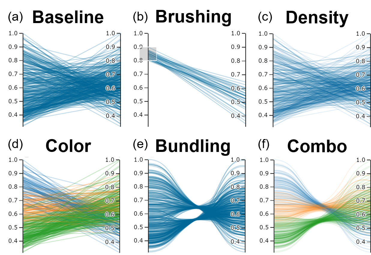
Due to the higher number of decision variables, we utilize parallel axis plots to identify how varying the decision variables can potentially affect certain performance objectives. Here, we use the regional reliability performance objective, REL, as an example. Figure 1 below demonstrates how all decision variables vary with regional reliability.

Figure 1: All decision variables for the three utilities. A darker blue indicates a higher degree of reliability.

From Figure 1, most solutions found via the optimization conducted in the previous blog post seem to have relatively high reliability across the full range of decision variable values. It is unclear as to how each decision variable might affect regional reliability. It is thus more helpful to identify specific sets of decision variables (or policies) that enable the achievement of reliability beyond a certain threshold.

With this in mind, we assume that all members of the Triangle require that their collective reliability be at least 98%. This results in the following figure:

Figure 2: All decision variables across the three utilities. The dark lines represent the policies that are at least 98% reliable.

Figure 2 has one clear takeaway: Pareto-optimality does not indicate satisfactory performance. In addition, setting this threshold make the effects of each decision variable clearer. It can be seen that regional reliability is significantly affected by both Durham and Raleigh’s infrastructure trigger (INF). Desirable levels of regional reliability can be achieved when Durham sets a high INF value. Conversely, Raleigh can set lower INF values to benefit from satisfactory reliability. Figure 2 also shows having Durham set a high insurance trigger (IT) may benefit the regional in terms of reliability.

However, there are caveats. Higher INF and IT values for Durham implies that the financial burden of investment and insurance payments are being borne by Raleigh and Cary, as Durham is able to withstand more risk without having to trigger an investment or infrastructure payment. This may affect how each member utility perceives their individual risks and benefits by forming a cooperative contract.

The code to plot these figures can be found under ‘refset_parallel.py’ in the repository.

Robustness analysis and what’s next

So how is setting a threshold value of regional reliability significant?

Within the MORDM framework, robustness is defined using a multivariate satisficing metric (Gold et al, 2019). Depending on the requirements of the stakeholders, a set of criteria is defined that will then be used distinguish between success (all criteria are met) and failure (at least one criteria is not met). Using these criteria, the rest of Pareto-optimal policies are simulated across a number of uncertain SOWs. Each policy’s robustness is then represented by the percent of SOWs in which it meets the minimum performance criteria that has been set.

In this post, we processed the reference set and visualized its decision variable space with respect to each variable’s effect on the reliability performance objective. A similar process can be repeated across all utilities for all performance objectives.

Using the processed reference set, we will conduct multi-criterion robustness analysis using two criteria:

1. Regional reliability should be at least 98%
2. Regional restriction frequency should be less than or equal to 20%

We will also conduct sensitivity analysis to identify the the decision variables that most impact regional robustness. Finally, we will conduct scenario discovery to identify SOWs that may cause the policies to fail.

References

Gold, D. F., Reed, P. M., Trindade, B. C., & Characklis, G. W. (2019). Identifying actionable compromises: Navigating multi‐city robustness conflicts to discover cooperative safe operating spaces for regional water supply portfolios. Water Resources Research, 55(11), 9024–9050. https://doi.org/10.1029/2019wr025462

Trindade, B. C., Reed, P. M., & Characklis, G. W. (2019). DEEPLY UNCERTAIN PATHWAYS: Integrated multi-city Regional Water Supply Infrastructure Investment and portfolio management. Advances in Water Resources, 134, 103442. https://doi.org/10.1016/j.advwatres.2019.103442

Parallel axis plots for the absolute beginner

A parallel axis plot is a simple way to convey a lot of information in a meaningful and easy-to-understand way. Also known as parallel coordinate plots (PCP), it is a visualization technique used to analyze multivariate numerical data (Weitz, 2020), or in the case of multi-objective optimization, to analyze tradeoffs between multiple conflicting objectives. As someone new to the field of multi-objective optimization, I found them particularly helpful as I tried to wrap my head around the multi-dimensional aspects of this field.

There are multiple tools in Python that you can use to generate PCPs. There are several different posts by Bernardo and Jazmin that utilize the Pandas and Plotting libraries to do so. In this post, I would like to explain a little about how you can generate a decent PCP using only Numpy and Matplotlib.

For context, I used a PCP to contrast the non-dominated solutions from the entire reference set of the optimized GAA problem reference set.

For the beginner, the figure above demonstrates three important visualization techniques in generating PCPs: color, brushing, and axis ordering. Firstly, it is important to consider using colors that stand on opposite sides on the color wheel to contrast the different types of information you are presenting. Next, brushing should be used to divert the viewer’s attention away from any information deemed unnecessary, highlight vital information, or to prove a point using juxtaposition. Finally, the ordering of the axes is important, particularly when presenting conflicting objectives. It is best for all axes to be oriented in one “direction of preference”, so that the lines between each adjacent axis can represent the magnitude of the tradeoff between two objectives. Thus, the order in which these axes are placed will significantly affect the way the viewer perceives the tradeoffs, and should be well-considered.

To help with understanding the how to generate a PCP, here is a step-by-step walk-through of the process.

1. Import all necessary libraries, load data and initialize the Matplotlib figure

import numpy as np
import matplotlib.pyplot as plt
from matplotlib import ticker

# load data
all_soln = np.loadtxt(open("GAA-reference-set.csv"), delimiter=",")
nd_indices = np.loadtxt(open("non-dominated-index.csv"), delimiter=",")

# identify and list the objectives of the reference set
objs = ['NOISE', 'WEMP', 'DOC', 'ROUGH', 'WFUEL', 'PURCH', 'RANGE', 'LDMAX', 'VCMAX', 'PFPF']

# create an array of integers ranging from 0 to the number of objectives                    
x = [i for i, _ in enumerate(objs)]

# sharey=False indicates that all the subplot y-axes will be set to different values
fig, ax  = plt.subplots(1,len(x)-1, sharey=False, figsize=(15,5))

Two sets of data are loaded:

• all_soln: the entire reference set
• nd_indices: an array of row indices of the non-dominated solutions from all_soln

In Line 16, we are initializing a figure fig and an array of axis objects ax. I find that having an array of axes helps me better control tick locations and labeling, since I can iterate over them in a loop.

Bear in mind that this is simply an example. It is also possible to obtain the non-dominated set directly from the the reference set by performing a Pareto sort.

2. Normalize the objective values in all_soln

min_max_range = {}

for i in range(len(objs)):
    all_soln[:,i] = np.true_divide(all_soln[:,i] - min(all_soln[:,i]), np.ptp(all_soln[:,i]))
    min_max_range[objs[i]] = [min(all_soln[:,i]), max(all_soln[:,i]), np.ptp(all_soln[:,i])]

All values in all_soln are normalized by subtracting the minimum value from each objective, then dividing it by the range of values for that objective. The min_max_range dictionary contains the minimum, maximum and range of values for each objective. This will come in handy later on.

3. Iterate through all the axes in the figure and plot each point

I used the enumerate function here. It may seem somewhat confusing at first, but it basically keeps count of your iterations as your are iterating through an object (ie: a list, an array). More information on how it works can be found here.

for i, ax_i in enumerate(ax):
    for d in range(len(all_soln)):
        if ((d in nd_indices)== False):
            if (d == 0):
                ax_i.plot(objs, all_soln[d, :], color='lightgrey', alpha=0.3, label='Dominated', linewidth=3)
            else:
                ax_i.plot(objs, all_soln[d, :], color='lightgrey', alpha=0.3, linewidth=3)
    ax_i.set_xlim([x[i], x[i+1]])

for i, ax_i in enumerate(ax):
    for d in range(len(all_soln)):
        if (d in nd_indices):
            if (d == nd_indices[0]):
                ax_i.plot(objs, all_soln[d, :], color='c', alpha=0.7, label='Nondominated', linewidth=3)
            else:
                ax_i.plot(objs, all_soln[d, :], color='c', alpha=0.7, linewidth=3)
    ax_i.set_xlim([x[i], x[i+1]])

All solutions from the non-dominated set are colored cyan, while the rest of the data is greyed-out. This is an example of brushing. Note that only the first line plotted for both sets are labeled, and that the grey-out data is plotted first. This is so the non-dominated lines are shown clearly over the brushed lines.

4. Write a function to position y-axis tick locations and labels

The set_ticks_for_axis() function is key to this process as it grants you full control over the labeling and tick positioning of your y-axes. It has three inputs:

• dim: the index of a value from the objs array
• ax_i: the current axis
• ticks: the desired number of ticks

def set_ticks_for_axis(dim, ax_i, ticks):
    min_val, max_val, v_range = min_max_range[objs[dim]]
    step = v_range/float(ticks)
    tick_labels = [round(min_val + step*i, 2) for i in range(ticks)]
    norm_min = min(all_soln[:,dim])
    norm_range = np.ptp(all_soln[:,dim])
    norm_step =(norm_range/float(ticks-1))
    ticks = [round(norm_min + norm_step*i, 2) for i in range(ticks)]
    ax_i.yaxis.set_ticks(ticks)
    ax_i.set_yticklabels(tick_labels)

Hello min_max_range! This dictionary essentially makes accessing the extreme values and range of each objective easier and less mistake-prone. It is optional, but I do recommend it.

Overall, this function does two things:

1. Creates ticks-evenly spaced tick-marks along ax_i.
2. Labels ax_i with tick labels of size ticks. The tick labels are evenly-spaced values generated by adding step*i to min_val for each iteration i.

A nice thing about this function is that is also preserves the order that the objective values should be placed along the axis, which makes showing a direction of preference easier. It will be used to label each y-axis in our next step.

5. Iterate over and label axes

for dim, ax_i in enumerate(ax):
    ax_i.xaxis.set_major_locator(ticker.FixedLocator([dim]))
    set_ticks_for_axis(dim, ax_i, ticks=10)

FixedLocator() is a subclass of Matplotlib’s ticker class. As it’s name suggests, it fixes the tick locations and prevents changes to the tick label or location that may possibly occur during the iteration. More information about the subclass can be found here.

Here, you only need to label the x-axis with one label and one tick per iteration (hence Line 2). On the other hand, you are labeling the entire y-axis of ax_i, which is where you need to use set_ticks_for_axis().

6. Create a twin axis on the last axis in ax

ax2 = plt.twinx(ax[-1])
dim = len(ax)
ax2.xaxis.set_major_locator(ticker.FixedLocator([x[-2], x [-1]]))
set_ticks_for_axis(dim, ax2, ticks=10)
ax2.set_xticklabels([objs[-2], objs[-1]])

Creating a twin axis using plt.twinx() enables you to label the last axis with y-ticks. Line 3 and 5 ensure that the x-axis is correctly labeled with the last objective name.

7. Finally, plot the figure

plt.subplots_adjust(wspace=0, hspace=0.2, left=0.1, right=0.85, bottom=0.1, top=0.9)
ax[8].legend(bbox_to_anchor=(1.35, 1), loc='upper left', prop={'size': 14})
ax[0].set_ylabel("$\leftarrow$ Direction of preference", fontsize=12)
plt.title("PCP Example", fontsize=12)
plt.savefig("PCP_example.png")
plt.show()

Be sure to remember to label the direction of preference, and one you’ve saved your plot, you’re done!

The source code to generate the following plot can be found here. I hope this makes parallel axis plots a little more understandable and less intimidating.

References

Weitz, D. (2020, July 27). Parallel Coordinates Plots. Retrieved November 09, 2020, from https://towardsdatascience.com/parallel-coordinates-plots-6fcfa066dcb3

Keen, B.A., Parallel Coordinates in Matplotlib. (2017, May 17). Retrieved November 09, 2020, from https://benalexkeen.com/parallel-coordinates-in-matplotlib/

Beyond Hypervolume: Dynamic visualization of MOEA runtime

Multi-objective evolutionary algorithms have become an essential tool for decision support in water resources systems. A core challenge we face when applying them to real world problems is that we don’t have analytic solutions to evaluate algorithmic performance, i.e. since we don’t know what solutions are possible before hand, we don’t have a point of reference to assess how well our algorithm is performing. One way we can gain insight into algorithmic performance is by examining runtime dynamics. To aid our understanding of the dynamics of the Borg MOEA, I’ve written a small Python library to read Borg runtime files and build a dynamic dashboard that visualizes algorithmic progress.

The Borg MOEA produces runtime files which track algorithmic parameters and the evolving Pareto approximate set over an optimization run. Often we use these data to calculate performance metrics, which provide information on the relative convergence of an approximation set and the diversity of solutions within it (for background on metrics see Joe’s post here). Commonly, generational distance, epsilon indicator and hypervolume are used to examine quality of the approximation set. An animation of these metrics for the 3 objective DTLZ2 test problem is shown in Figure 1 below.

Figure 1: Runtime metrics for the DTLZ2 test problem. The x-axis is number of function evaluations, the y-axis is the each individual metric

While these metrics provide a helpful picture of general algorithmic performance, they don’t provide insight into how the individual objectives are evolving or Borg’s operator dynamics.

Figure 2 shows a diagnostic dashboard of the same 3 objective DTLZ2 test problem run. I used the Celluloid python package to animate the figures. I like this package because it allows you to fully control each frame of the animation.

Figure 2: DTLZ2 runtime dynamics. The tree objectives are shown in a scatter plot and a parallel axis plot. The third figure plots hypervolume over the optimization run and the bottom figure shows Borg’s operator dynamics. (a higher resolution version of this file can be found here: https://www.dropbox.com/s/0nus5xhwqoqtghk/DTLZ2_runtime.gif?dl=0)

One thing we can learn from this dashboard is that though hypervolume starts to plateau around 3500 NFE, the algorithm is still working to to find solutions that represent an adequately diverse representation of the Pareto front. We can also observe that for this DTLZ2 run, the SPX and SBX operators were dominant. SBX is an operator tailored to problems with independent decision variables, like DTLZ2, so this results make sense.

I’m planning on building off this dashboard to include a broader suite of visualization tools, including pairwise scatter plots and radial plots. The library can be found here: https://github.com/dgoldri25/runtimeDiagnostics

If anyone has suggestions or would like to contribute, I would love to hear from you!

Parasol: an open source, interactive parallel coordinates library for multi-objective decision making

For my entire graduate student career, I’ve gravitated toward parallel coordinates plots… in theory. These plots scale well for high-dimensional, multivariate datasets (Figure 1); and therefore, are ideal for visualizing multi-objective optimization solutions. However, I found it difficult to create parallel coordinates plots with the aesthetics and features I wanted.

Figure 1. An example parallel coordinates plot that visualizes the “cars” dataset. Each polyline represents the attributes of a particular car and similar types of cars have the same color polyline.

I was amazed when I learned about Parcoords–a D3-based parallel coordinates library for creating interactive web visualizations. D3 (data-driven documents) is a popular JavaScript library which offers developers total control over their visualizations. Building upon D3, the Parcoords library is capable of creating beautiful, functional, and shareable parallel coordinates visualizations. Bernardo (@bernardoct), David (@davidfgold), and Jan Kwakkel saw the potential of Parcoords, each developing tools (tool #1 and tool #2) and additional features. Exploring these tools, I liked how they linked parallel coordinates plots with interactive data tables using the SlickGrid library. Being able to inspect individual solutions was so powerful. Plus, the features in Parcoords like interactive brushing, reorderable axes, easy-to-read axes labels, blew my mind. Working with large datasets was suddenly intuitive!

The potential of these visualizations was inspiring, but learning web development (i.e., JavaScript, CSS, and HTML) was daunting. Not only would I have to learn web development, I would need to learn how to use multiple libraries, and figure out how to link plots and tables together to make these types of tools. It just seemed like too much work for this sort of visualization to catch on… and that was the inspiration behind Parasol. Together with my advisor (Joe Kasprzyk, @jrk301) and Josh Jacobson, we built Parasol to streamline the development of linked, web-based parallel coordinates visualizations.

We’ve published a paper describing the Parasol library in Environmental Modelling & Software, so please refer to that paper for an in-depth discussion:

Raseman, William J., Joshuah Jacobson, and Joseph R. Kasprzyk. “Parasol: An Open Source, Interactive Parallel Coordinates Library for Multi-Objective Decision Making.” Environmental Modelling & Software 116 (June 1, 2019): 153–63. https://doi.org/10.1016/j.envsoft.2019.03.005.

In this post, I’ll provide a brief, informal overview of Parasol’s features and some example applications.

Cleaning up the clutter with Parasol

Parallel coordinates can visualize large, high-dimensional datasets, but at times they can become difficult to read when polylines overlap and obscure the underlying data. This issue is known as “overplotting” (see Figure 1 and 2a). That’s why we’ve implemented a suite of “clutter reduction techniques” in Parasol that enables the user to tidy up the data dynamically.

Probably the most powerful clutter reduction technique is brushing (Figure 2b). Using interactive filters, the user can filter out unwanted data and focus on a subset of interest. Users can also alter polyline transparency to reveal density in the data (Figure 2c), assign colors to polylines (Figure 2d), and apply “curve bundling” to group similar data together in space (Figure 2e). These clutter reduction techniques can also be used simultaneously to enhance the overall effect (Figure 2f).

Figure 2. Vanilla parallel coordinates plots (a) suffer from “overplotting”, obscuring the underlying data. Interactive filters (b: brushes) and other clutter reduction techniques (c-f) alleviate these issues.

Another cool feature of both Parcoords and Parasol is dynamically reorderable axes (Figure 3). With static plots, the user can only look at pairwise relationships between variables plotted on adjacent axes. With reorderable axes, they are free to explore any pairwise comparison they choose!

Figure 3. Users can click and drag axes to interactively reorder them.

API resources

The techniques described above (and many other features) are implemented using Parasol’s application programming interface (API). In the following examples (Figures 4-6), elements of the API are denoted using ps.XXX(). For a complete list of Parasol features, check out the API Reference on the Parasol GitHub repo.

Example applications

The applications (shown in Figures 4-6) demonstrate the library’s ability to create a range of custom visualization tools. To open the applications, click on the URL in the caption below each image and play around with them for yourself. Parallel coordinates plots are meant to be explored!

Figure 4. Example app #1: https://parasoljs.github.io/demo/paper-example-1.html

Example app #1 (Figure 4) illustrates the use of linked parallel coordinates plots. If the user applies a brush on one plot, the changes will be reflected on both linked plots. Furthermore, app developers can embed functionalities of the Parasol API using HTML buttons. For instance, if the user applies multiple brushes to the plots, they can reset all the brushes by clicking on the “Reset Brushes” button which invokes ps.resetSelections(). Other functionalities allow the user to remove the brushed data from a plot [ps.removeData()] or keep only the brushed data [ps.keepData()] and export brushed data [ps.exportData()].

Figure 5. Example app #2: https://parasoljs.github.io/demo/paper-example-2.html

Example app #2 (Figure 5) demonstrates utility of linking data tables to parallel coordinates plots. By hovering a mouse over a data table row, the corresponding polyline will become highlighted. This provides the user with the ability to fine-tune their search and inspect individual data points–a rare feature in parallel coordinates visualizations.

App #2 also demonstrates how k-means clustering [ps.cluster()] can enhance these visualizations by sorting similar data into groups or clusters. In this example, we denote the clusters using color. Using a slider, users can alter the number of clusters (k) in real-time. Using checkboxes, they can customize which variables are included in the clustering calculation.

Figure 6. Example app #3: https://parasoljs.github.io/demo/paper-example-3.html

Example app #3 also incorporates clustering but encodes the clusters using both color and “curve bundling”. With curve bundling, polylines in the same cluster are attracted to one another in the whitespace between the axes. Bundling is controlled by two parameters: 1) curve smoothness and 2) bundling strength. This app allows the user to play around with these parameters using interactive sliders.

Similar to highlighting, Parasol features “marking” to isolate individual data points. Highlighting is temporary, when the user’s mouse leaves the data table, the highlight will disappear. By clicking a checkbox on the data table, the user can “mark” data of interest for later. Although marks are more subtle than highlights, they provide a similar effect.

Lastly, this app demonstrates the weighted sum method [ps.weightedSum()]. Although we don’t generally recommend aggregating objectives in multi-objective optimization literature, there are times when assigning weights to different variables and calculating an aggregate score can be useful. In the above example, the user can input different combinations of weights with text input or using sliders.

We want to hear from you!

For the most up-to-date reference on Parasol, see the GitHub repo, and for additional examples, check out the Parasol webpage. We would love to hear from you, especially if you have suggestions for new features or bugs to report. To do so, post on the issues page for the repo.

If you make a Parasol app and want to share it with the world, post a link in the comments below. It would be great to see what people create!

Parasol tutorials

If you aren’t sure how to start developing Parasol applications, don’t worry. In subsequent posts, I’ll take you step-by-step through how to make some simple apps and give you the tools to move on to more complicated, custom applications.

Those tutorials are currently under development and can be found on the Parasol GitHub wiki.