This post is an account of my recent experience with Google Earth Pro (GPE), a free online tool meant to make visualization of geographical information intuitive and accessible. This account contains tidbits that I thought others might find useful, but it is not meant to be an unbiased or comprehensive resource.
My goal in using GPE was to set up a short video tour of the reservoirs on the main stem of the Upper Snake River, which has its upper reaches around the Teton Range (WY, USA) before going through much of southern Idaho. Here is the video, produced with instructions from this post from the blog:
The cool
GPE is indeed an intuitive way for people that have only a limited experience of geographic information systems (GIS) to put together nice-looking videos in a limited amount of time. It relies on the increasingly large amounts of geographic data available online. For instance, polygons made of points with geographical coordinates, used to delineate political boundaries or catchments among others, can be found increasingly easily, be it under formats specific to GPE (KML, KMZ), or traditional GIS format such as SHP (shapefile format, which can be imported to GPE with… “File => Import”, I told you it was intuitive). This capability to find the right data could be improved by the recent launch of a dataset search engine by Google.
This video, after several tests, superposed three layers on the satellite images of the land surface:
Pins of the dams’ locations. Please refer to this post to learn all you need to know about setting and customizing such new placemarks.
The network of all streams with an average flow of more than 10 m3/s in the Columbia River basin. This is mainly for easy visualization of where the Snake River and its affluents are. That data was obtained from this useful USGS resource, with all the major basins in the US having data in GPE-ready KML format (basin boundaries, tributaries with their average flows, landuse, etc.).
An invisible layer contains the shapes of the reservoirs’ lakes, in order to zoom in on the reservoir and not the dam itself. I got the shapes of waterbodies in the Upper Snake River basin from an amazing resource for water resources practitioners (see “The limits” below to see how to access this resource, but also to understand why it must be handled with care). Hint: since the list of waterbodies is dauntingly large and includes every little puddle in the area, I had to zoom in to the desired reservoir so as to only select its shape, by doing “File => Import”, then when prompted, by choosing to only import the features in my line of sight.
The trade-offs
The trade-offs when doing this kind of short intro video to your study area, are between video quality and required memory. This is especially true if the video is of a rather large area, as the GPE satellite images embed a level of detail that is amazing at the scale of that basin. Therefore, when creating my video, I had to resort to several tries before getting a correct quality, and this video eats up 500Mo of disk space for 43 seconds (!!!!). Any video with lower resolution just looked downright disgusting, whereas any larger video may have serious problem running on your laptop. Think of it as a Goldilocks zone that you have to find if you want to have a video you can embed in an oral presentation.
(NB: to embed this video in a presentation in a fullproof kind of way, the easiest is to embed a link from the PPT file to the video in the same folder).
The limits
The limits of Google Earth are with its plain refusal to display features it deems too big. To understand this, let us look at this USGS webpage where a sizable of hydrological information can be downloaded. In particular it is possible to download data exactly for the upper Snake area (Subregion 1704 on the picture below). This data can include waterbodies as discussed above (in “the cool”) and that is contained in the NHD data ticket in the picture. By ticking “Watershed Boundary Dataset (WBD)”, one can also download basin and subbasin boundaries.
Why then did I not represent Upper Snake boundaries in my video? Well, the Upper Snake polygon, under SHP format at least, is too big so GPE just… refused to display it. I tried to represent the HU-6 and HU-8 subbasins (smaller than the HU-4-sized Upper Snake under this classification system, and:
The HU-6 subbasin just divides the basin into “headwaters” (smaller part upstream of Palisades) and “the rest”; the former feature was smaller and GPE plotted it, but it did not plot the latter.
The HU-8 subbasins all are individually smaller features that GPE accepts to plot. So I could have plotted the watershed boundaries by plotting ALL of the HU-8 subbasins, but spoiler alert: this looked horrendous.
Takeaway: GPE only displays features that individually have limited size. So maybe using a more powerful and recent desktop computer than the one I had would have done the trick… but be aware that there will always be a limit. Also note that assuming that GPE is just taking its time loading the data, and that staring blankly at the screen in the meantime is not going to be too painful, is not a good idea. Take a nap instead, or do something else, then admit that the damn thing just did not display.
A solution for this, of course, is to load the larger features on GIS software and making them lighter by eliminating points in the polygon without altering the shape… but that kinda beats the purpose of GPE, which is to avoid having to become a GIS geek, doesn’t it?
Python libraries can be very helpful in making visualizations. One particular library I like using is the Bokeh library. In this post, I will share how this library can be used for visualizing trade offs across multiple objectives.
First import the libraries we need for our plots:
import pandas as pd
from bokeh.io import output_file, show #for outputting and showing plots
from bokeh.plotting import figure #for creating figures, which are the plot area in this case
from bokeh.models.tools import HoverTool #for importing the hover tool
from bokeh.models import ColumnDataSource #which we will ultimately use for linking plots
from bokeh.models.widgets import Panel, Tabs #for making tabs
Basic Plotting
Let’s start by creating a basic plot for a three objective DTLZ2, where the first and second objectives are plotted on the x and y axes respectively, and the third objective is the size of the plotted points.
# create a new plot using the figure function
p = figure(title="DTLZ2 with 3 objectives",plot_width=400, plot_height=400)

# add axis titles
p.xaxis.axis_label = "Objective 1"
p.yaxis.axis_label = "Objective 2"

# upload your data
paretoFront = pd.read_csv("C:/Users/Sarah/Desktop/dmh309-serial-borg-moea-2c7702638d42/dtlz2obj.csv")

# assign data to arrays
obj1=paretoFront['Obj1']
obj2=paretoFront['Obj2']
obj3=paretoFront['Obj3']

# plots points
paretoPlot = p.circle(obj1, obj2, size=obj3*10, # objective 3 is the shown by the size of the points; I multiplied by 10 to make them clearer
       fill_color="grey", # for more color options, check out https://bokeh.pydata.org/en/latest/docs/reference/colors.html
       fill_alpha=0.6, # alpha is the transparency of the points
       line_color=None) # line_color is the outline of the points

# show the results
show(p)
The figure below shows what your plot will look like. Notice the default tools that are outlined on the right of the plot.
More useful tools
Although Bokeh plots come with a default set of useful tools, there are other tools which you could add to make your plots more interactive.
To demonstrate some of these useful tools, I will create a figure with three tabs. Each tab will contain a view of the Pareto front for two of the three objectives. In addition, these tabs will be linked, so that if you make a selection on the Pareto front in one of the tabs, the same points will be selected in the other views. I will also demonstrate the use of the vertical, horizontal, and mouse over hover tools, and add data labels for the mouse over hover tool.
paretoFront = pd.read_csv("C:/Users/Sarah/Desktop/dmh309-serial-borg-moea-2c7702638d42/dtlz2obj_reduced.csv")

obj1=paretoFront['Obj1']
obj2=paretoFront['Obj2']
obj3=paretoFront['Obj3']

# create a column data source for the plots; this will allow us to link the plots we create
source = ColumnDataSource(data=dict(x=obj1, y=obj2, z=obj3))

# define the tools you want to use; if you are defining tools, you need to list all the tools you want, including the default Bokeh tools
TOOLS = "box_select,lasso_select,help,pan,wheel_zoom,box_zoom,reset,save"

# create a new plot for each view/tab using figure
p1 = figure(tools=TOOLS,title="DTLZ2 (Objective 1, Objective 2)",plot_width=400, plot_height=400)
p2 = figure(tools=TOOLS,title="DTLZ2 (Objective 1, Objective 3)",plot_width=400, plot_height=400)
p3 = figure(tools=TOOLS,title="DTLZ2 (Objective 2, Objective 3)",plot_width=400, plot_height=400)

# define functions for hovering
def verticalhover(p,paretoPlot):
    p.add_tools(HoverTool(tooltips=None, renderers=[paretoPlot], mode='vline'))

def horizontalhover(p,paretoPlot):
    p.add_tools(HoverTool(tooltips=None, renderers=[paretoPlot], mode='hline'))

def pointhover(p, paretoPlot, obja, objb):
    p.add_tools(HoverTool(tooltips=[(obja, "$x" ), (objb, "$y")],mode="mouse", point_policy="follow_mouse", renderers=[paretoPlot]))
# note that we added 'tooltips' here, this gives the values (like excel data labels) of the points when you hover over them

# plot 1
paretoPlot1 = p1.circle('x', 'y',
                        fill_color='grey',
                        fill_alpha=0.7,
                        hover_fill_color="crimson", hover_alpha=0.8, # this changes the color and transparecy of the points when we hover over them
                        line_color=None, hover_line_color="white", source=source) # we will use 'source' in all our plots, because we want to link them by having them share the same sources data

p1.xaxis.axis_label = "Objective 1"
p1.yaxis.axis_label = "Objective 2"

# add the hover tools
verticalhover(p1,paretoPlot1)
horizontalhover(p1,paretoPlot1)
pointhover(p1, paretoPlot1, "objective 1", "objective 2")

# add the panel for the first tab
tab1 = Panel(child=p1, title="obj1, obj2")

# repeat the same steps for tabs 2 and 3 (i.e. objective 1 vs. objective 3 and objective 2 vs. objective 3)
# plot 2

paretoPlot2 = p2.circle('x','z',
                        fill_color='grey', hover_fill_color="crimson",
                        fill_alpha=0.7, hover_alpha=0.8,
                        line_color=None, hover_line_color="white", source=source)

p2.xaxis.axis_label = "Objective 1"
p2.yaxis.axis_label = "Objective 3"

verticalhover(p2,paretoPlot2)
horizontalhover(p2,paretoPlot2)
pointhover(p2, paretoPlot2, "objective 1", "objective 3")

tab2 = Panel(child=p2, title="obj1, obj3")

# plot 3

paretoPlot3 = p3.circle('y', 'z',
                        fill_color='grey', hover_fill_color="crimson",
                        fill_alpha=0.7, hover_alpha=0.8,
                        line_color=None, hover_line_color="white", source=source)

p3.xaxis.axis_label = "Objective 2"
p3.yaxis.axis_label = "Objective 3"

verticalhover(p3,paretoPlot3)
horizontalhover(p3,paretoPlot3)
pointhover(p3, paretoPlot3, "objective 2", "objective 3")

tab3 = Panel(child=p3, title="obj2, obj3")

# finally create the tabs and show your plot!
tabs = Tabs(tabs=[ tab1, tab2, tab3 ])
show(tabs)
The figure below shows the plot you will obtain:
Now, let’s explore the tools that we added:
Selection across multiple tabs: use lasso or box select to select some points in your first tab. When you move to the second and third tabs, the same points will be selected in different views.
Vertical and Horizontal Hover: select either the vertical or horizontal hover tool from the right toolbar. Make sure you deselect all other tools. The vertical hover will color in all the points that lie in the vertical line that crosses the point you are hovering over, and the horizontal hover does the same thing horizontally.
Point Hover and Data Labels: Select the point hover tool, deselect all the other tools, and hover over the points. When you hover over a point, you will get the values for the objectives for that point.
In this post, I will cover the very basics of Gaussian Processes following the presentations in Murphy (2012) and Rasmussen and Williams (2006) — though hopefully easier to digest. I will approach the explanation in two ways: (1) derived from Bayesian Ordinary Linear Regression and (2) derived from the definition of Gaussian Processes in functional space (it is easier than it sounds). I am not sure why the mentioned books do not use “^” to denote estimation (if you do, please leave a comment), but I will stick to their notation assuming you may want to look into them despite running into the possibility of an statistical sin. Lastly, I would like to thank Jared Smith for reviewing this post and providing highly statistically significant insights.
If you are not familiar with Bayesian regression (see my previous post), skip the section below and begin reading from “Succinct derivation of Gaussian Processes from functional space.”
From Bayesian Ordinary Linear Regression to Gaussian Processes
where we are trying to regress a model over the data set , being the independent variables and the dependent variable, is a vector of model parameters and is the model error variance. The unusual notation for the normal distribution means “a normal distribution of with (or given) the regression mean and variance ,” where is the number of points in the data set. The estimated variance of , and the estimated regression parameters can be calculated as
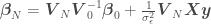
where and are the mean and the covariance of the parameter prior distribution. All the above can be used to estimate as
with an error variance of
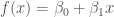
If we assume a prior mean of 0 (), replace and by their definitions, and apply a function , e.g. , to add features to so that we can use a linear regression approach to fit a non-linear model over our data set , we would instead have that
where and . One problem with this approach is that as we add more terms (also called features) to function to better capture non-linearities, the the dimension of the matrix we will have to invert increases. It is also not always obvious what features we should add to our data. Both problems can be handled with Gaussian Processes.
Now to Gaussian Processes
This is where we transition from Bayesian OLR to Gaussian Processes. What we want to accomplish in the rest of this derivation is to find a way of: (1) adding as many features to the data as we need to calculate and without increasing the size of the matrix we have to invert (remember the dimensions of such matrix equals the number of features in ), and of (2) finding a way of implicitly adding features to and without having to do so manually — manually adding features to the data may take a long time, specially if we decide to add (literally) an infinite number of them to have an interpolator.
The first step is to make the dimensions of the matrix we want to invert equal to the number of data points instead of the number of features in . For this, we can re-arrange the equations for and as
We now have our feature-expanded data and points for which we want point estimates always appearing in the form of — is just another point either in the data set or for which we want to estimate . From now on, will be called a covariance or kernel function. Since the prior’s covariance is positive semi-definite (as any covariance matrix), we can write
where . Using and assuming a prior of , and then take a new shape in the predictor posterior of a Gaussian Process:
where , and . Now the features of the data are absorbed within the inner-products between observed ‘s and or for , so we can add as many features as we want without impacting the dimensions of the matrix we will have to invert. Also, after this transformation, instead of and representing the mean and covariance between model parameters, they represent the mean and covariance of and among data points and/or points for which we want to get point estimates. The parameter posterior from Bayesian OLR would now be used to sample the values of directly instead of model parameters. And now we have a Gaussian Process with which to estimate . For plots of samples of from the prior and from the predictive posterior, of the mean plus or minus the error variances, and of models with different kernel parameters, see figures at the end of the post.
Kernel (or Covariance) matrices
The convenience of having and written in terms of , is that does not have to represent simply a matrix-matrix or vector-matrix multiplication of and . In fact, function can be any function that corresponds to an inner-product after some transformation from , which will necessarily return a positive semi-definite matrix and therefore be a valid covariance matrix. There are several kernels (or kernel functions or kernel shapes) available, each accounting in a different way for the nearness or similarity (at least in Gaussian Processes) between values of :
the linear kernel: . This kernel is used when trying to fit a line going through the origin.
the polynomial kernel: , where d is the dimension of the polynomial function. This kernel is used when trying to fit a polynomial function (such as the fourth order polynomial in the blog post about Bayesian OLR), and
the Radial Basis Function, or RBF (aka Squared Exponential, or SE), , where is a kernel parameter denoting the characteristic length scale of the function to be approximated. Using the RBF kernel is equivalent to adding an infinite (!) number of features the data, meaning .
But this is all quite algebraic. Luckily, there is a more straight-forward derivation shown next.
Succinct derivation of Gaussian Processes from functional space.
Most regression we study in school is a way of estimating the parameters of a model. In Bayesian OLR, for example, we have a distribution (the parameter posterior) from which to sample model parameters. What if we instead derived a distribution from which to sample functions themselves? The first (and second and third) time I heard about the idea of sampling functions I thought right away of opening a box and from it drawing exponential and sinusoid functional forms. However, what is meant here is a function of an arbitrary shape without functional form. How is this possible? The answer is: instead of sampling a functional form itself, we sample the values of at discrete points, with a collection of for all in our domain called a function . After all, don’t we want a function more often than not solely for the purpose of getting point estimates and associated errors for given values of ?
In Gaussian Process regression, we sample functions from a distribution by considering each value of in a discretized range along the x-axis as a random variable. That means that if we discretize our x-axis range into 100 equally spaced points, we will have 100 random variables . The mean of all possible functions at therefore represents the mean value of in , and each term in the covariance matrix (kernel matrix, see “Kernel (or Covariance) matrices” section above) represents how similar the values of and will be for each pair and based on the value of a distance metric between and : if and are close to each other, and tend to be similar and vice-versa. We can therefore turn the sampled functions into whatever functional form we want by choosing the appropriate covariance matrix (kernel) — e.g. a linear kernel will return a linear model, a polynomial kernel will return a polynomial function, and an RBF kernel will return a function with an all linear and an infinite number of non-linear terms. A Gaussian Process can then be written as
where is the mean function (e.g. a horizontal line along the x-axis at y = 0 would mean that ) and is the covariance matrix, which here expresses how similar the values of will be based on the distance between two values of .
To illustrate this point, assume we want to sample functions over 200 discretizations along the x-axis from x=-5 to x=5 () using a Gaussian Process. Assume the parameters of our Gaussian Process from which we will sample our functions are mean 0 and that it uses an RBF kernel for its covariance matrix with parameter (not be confused with standard deviation), meaning that and , or
Each sample from the normal distribution above will return 200 values: . A draw of 3 such sample functions would look generally like the following:
The functions above look incredibly smooth because of the RBF kernel, which adds an infinite number of non-linear features to the data. The shaded region represents the prior distribution of functions. The grey line in the middle represents the mean of an infinite number of function samples, while the upper and lower bounds represent the corresponding prior mean plus or minus standard deviations.
These functions looks quite nice but pretty useless. We are actually interested in regressing our data assuming a prior, namely on a posterior distribution, not on the prior by itself. Another way of formulating this is to say that we are interested only in the functions that go through or close to certain known values of and . All we have to do is to add random variables corresponding to our data and condition the resulting distribution on them, which means accounting only for samples of functions that exactly go through (or given) our data points. The resulting distribution would then look like . After adding our data , or , our distribution would look like
In this distribution we have random variables representing the from our data set and the from which we want to get point estimates and corresponding error standard deviations. The covariance matrix above accounts for correlations of all observations with all other observations, and correlations of all observations with all points to be predicted. We now just have to condition the multivariate normal distribution above over the points in our data set, so that the distribution accounts for the infinite number of functions that go through our at the corresponding . This yields
where , , , and is a vector containing the elements in the diagonal of the covariance matrix — the variances of each random variable . If you do not want to use a prior with , the mean of the Gaussian Process would be . A plot of estimated for 200 values of — so that the resulting curve looks smooth — plus or minus associated uncertainty (), regressed on 5 random data points , , should look generally like
A plot of three sampled functions (colored lines below, the grey line is the mean) should look generally like
Several kernel have parameters that can strongly influence the regressed model and that can be estimated — see Murphy (2012) for a succinct introduction to kernel parameters estimation. One example is parameter of the RBF kernel, which determines the correlation length scale of the fitted model and therefore how fast with increasing separation distance between data points the model will default to the prior (here, with ). The figure below exemplifies this effect
All figures have the same data points but the resulting models look very different. Reasonable values for depend on the spacing between the data points and are therefore data-specific. Also, if when you saw this plot you thought of fitting RBF functions as interpolators, that was not a coincidence: the equations solved when fitting RBFs to data as interpolators are the same solved when using Gaussian Processes with RBF kernels.
Lastly, in case of noisy observation of in the Gaussian Process distribution and the expressions for the mean, covariance, and standard deviation become
where is the error variance and is an identity matrix. The mean and error predictions would look like the following
Concluding Remarks
What I presented is the very basics of Gaussian Processes, leaving several important topics which were not covered here for the interested reader to look into. Examples are numerically more stable formulations, computationally more efficient formulations, kernel parameter estimation, more kernels, using a linear instead of zero-mean prior (semi-parametric Gaussian Processes), Gaussian Processes for classification and Poisson regression, the connection between Gaussian Processes and other methods, like krieging and kernel methods for nonstationary stochastic processes. Some of these can be found in great detail in Rasmussen and Williams (2006), and Murphy (2012) has a succinct presentation of all of the listed topics.
I was really confused about Gaussian Processes the first time I studied it and tried to make this blog post as accessible as possible. Please leave a comment if you think the post would benefit from any particular clarification.
References
Murphy, Kevin P., 2012. Machine Learning: A Probabilistic Perspective. The MIT Press, ISBN 978-0262018029
Rasmussen, Carl Edward and Williams, Christopher K. I., 2006. Gaussian Processes for Machine Learning. The MIT Press, ISBN 978-0262182539.
This semester I am teaching Engineering Management Methods here at Cornell University. The course is aimed at introducing engineering students to systems thinking and a variety of tools and analyses they can use to analyze data. The first chapter has been on time series forecasting, where we discussed some of the simpler models one can use and apply for forecasting purposes, including Simple and Weighted Moving Average, Single and Double Exponential Smoothing, Additive and Multiplicative Seasonal Models, and Holt Winter’s Method.
The class applications as well as the homework are primarily performed in Excel, but I have been trying, with limited success, to encourage the use of programming languages for the assignments. One comment I’ve received by a student has been that it takes significantly more time to perform the calculations by coding; they feel that it’s a waste of time. I initially attributed the comment to the fact that the student was new to coding and it takes time in the beginning, but on later reflection I realized that, in fact, the student was probably simply manually repeating the same Excel operations by using code: take a set of 30 observations, create an array to store forecasts, loop through every value and calculate forecast using model formula, calculate error metrics, print results, repeat steps for next set of data. It occurred to me that of course they think it’s a waste of time, because doing it that way completely negates what programming is all about: designing and building an executable program or function to accomplish a specific computing task. In this instance, the task is to forecast using each of the models we learn in class and the advantage of coding comes with the development of some sort of program or function that performs these operations for us, given a set of data as input. Simply going through the steps of performing a set of calculations for a problem using code is not much different than doing so manually or in Excel. What is different (and beneficial) is designing a code so that it can then be effortlessly applied to all similar problems without having to re-perform all calculations. I realize this is obvious to the coding virtuosos frequenting this blog, but it’s not immediately obvious to the uninitiated who are rather confused on why Dr. Hadjimichael is asking them to waste so much time for a meager bonus on the homework.
So this blog post, is aimed at demonstrating to coding beginners how one can transition from one way of thinking to the other, and providing a small time-series-forecasting toolkit for users that simply want to apply the models to their data.
The code and data for this example can be found on my GitHub page and I will discuss it below. I will be using a wine sales dataset that lists Australian wine sales (in kiloliters) from January 1980 to October 1991. The data looks like this:
This file contains bidirectional Unicode text that may be interpreted or compiled differently than what appears below. To review, open the file in an editor that reveals hidden Unicode characters.
Learn more about bidirectional Unicode characters
We first need to import the packages we’ll be using and load the data. I will be using Pandas in this example (but there’s other ways). I’m also defining the number of seasonal periods in a cycle, in this case 12.
import numpy as np #Package we'll use for numerical calculations
import matplotlib.pyplot as plt #From matplotlib package we import pyplot for plots
import pandas #Package to data manipulation
import scipy.optimize #Package we'll use to optimize
plt.style.use('seaborn-colorblind') #This is a pyplot style (optional)

'''Load the data into a pandas series with the name wine_sales'''
time_series = pandas.Series.from_csv("wine_sales.csv", header=0)

P=12 #number of seasonal periods in a cycle
In class, I’ve always mentioned that one should use a training and a validation set for model development, primarily to avoid overfitting our model to the specific training set. In this example, the functions are written as they apply to the training set. Should you choose to apply the functions listed here, you should apply the functions for the training set, extract forecasts and then use those to initialize your validation period. To divide the observations, you would do something like this:
training = time_series[0:108] # Up to December '88
validation = time_series[108:] # From January '89 until end
Now, if say, we wanted to apply the Naive model of the next steps forecast being equal to the current observation, i.e., , we’d do something like:
y_hat=pandas.Series().reindex_like(time_series) # Create an array to store forecasts
y_hat[0]= time_series[0] # Initialize forecasting array with first observation
''' Loop through every month using the model to forecast y_hat'''
for t in range(len(y_hat)-1): # Set a range for the index to loop through
    y_hat[t+1]= time_series[t] # Apply model to forecast time i+1
Now if we’d like to use this for any time series, so we don’t have to perform our calculations every time, we need to reformat this a bit so it’s a function:
def naive(time_series):
    y_hat=pandas.Series().reindex_like(time_series)
    y_hat[0]= time_series[0] # Initialize forecasting array with first observation
    ''' Loop through every month using the model to forecast y'''
    #This sets a range for the index to loop through
    for t in range(len(y_hat)-1):
        y_hat[t+1]= time_series[t] # Apply model to forecast time i+1
    return y_hat
Now we can just call define this function at the top of our code and just call it with any time series as an input. The function as I’ve defined it returns a pandas.Series with all our forecasts. We can then do the same for all the other modeling methods (below). Some things to note:
The data we read in the top, outside the functions, as well as any parameters defined (P in this case) are global variables and do not need to be defined as an input to the function. The functions below only need a list of parameter values as inputs.
For the models with seasonality and/or trend we need to create separate series to store those estimates for E, S, and T.
Each model has its own initialization formulas and if we wanted to apply them to the validation set that follows our training set, we’d need to initialize with the last values of our training.
'''SIMPLE MOVING AVERAGE
Using this model, y_hat(t+1)=(y(t)+y(t-1)...+y(t-k+1))/k (i.e., the predicted
next value is equal to the average of the last k observed values).'''
def SMA(params):
    k=int(np.array(params))
    y_hat=pandas.Series().reindex_like(time_series)
    y_hat[0:k]=time_series[0:k]
    ''' Loop through every month using the model to forecast y.
    Be careful with Python indexing!'''
    for t in range(k-1,len(y_hat)-1): #This sets a range for the index to loop through
        y_hat[t+1]= np.sum(time_series[t-k+1:t+1])/k # Apply model to forecast time i+1
    return y_hat

'''WEIGHTED MOVING AVERAGE
Using this model, y_hat(t+1)=w(1)*y(t)+w(2)*y(t-1)...+w(k)*y(t-k+1) (i.e., the
predicted next value is equal to the weighted average of the last k observed
values).'''
def WMA(params):
    weights = np.array(params)
    k=len(weights)
    y_hat=pandas.Series().reindex_like(time_series)
    y_hat[0:k]=time_series[0:k] # Initialize values
    ''' Loop through every month using the model to forecast y.
    Be careful with Python indexing!'''
    for t in range(k-1,len(y_hat)-1): #This sets a range for the index to loop through
        y_hat[t+1]= np.sum(time_series[t-k+1:t+1].multiply(weights)) # Apply model to forecast time i+1
    return y_hat
'''This model includes the constraint that all our weights should sum to one.
To include this in our optimization later, we need to define it as a function of our
weights.'''
def WMAcon(params):
    weights = np.array(params)
    return np.sum(weights)-1

'''SINGLE EXPONENTIAL SMOOTHING
Using this model, y_hat(t+1)=y_hat(t)+a*(y(t)-y_hat(t))(i.e., the
predicted next value is equal to the weighted average of the last forecasted value and its
difference from the observed).'''
def SES(params):
    a = np.array(params)
    y_hat=pandas.Series().reindex_like(time_series)
    y_hat[0]=time_series[0] # Initialize values
    ''' Loop through every month using the model to forecast y.
    Be careful with Python indexing!'''
    for t in range(len(y_hat)-1): #This sets a range for the index to loop through
        y_hat[t+1]=  y_hat[t]+a*(time_series[t]-y_hat[t])# Apply model to forecast time i+1
    return y_hat

'''DOUBLE EXPONENTIAL SMOOTHING (Holts Method)
Using this model, y_hat(t+1)=E(t)+T(t) (i.e., the
predicted next value is equal to the expected level of the time series plus the
trend).'''
def DES(params):
    a,b = np.array(params)
    y_hat=pandas.Series().reindex_like(time_series)
    '''We need to create series to store our E and T values.'''
    E = pandas.Series().reindex_like(time_series)
    T = pandas.Series().reindex_like(time_series)
    y_hat[0]=E[0]=time_series[0] # Initialize values
    T[0]=0
    ''' Loop through every month using the model to forecast y.
    Be careful with Python indexing!'''
    for t in range(len(y_hat)-1): #This sets a range for the index to loop through
        E[t+1] = a*time_series[t]+(1-a)*(E[t]+T[t])
        T[t+1] = b*(E[t+1]-E[t])+(1-b)*T[t]
        y_hat[t+1] = E[t] + T[t] # Apply model to forecast time i+1
    return y_hat

'''ADDITIVE SEASONAL
Using this model, y_hat(t+1)=E(t)+S(t-p) (i.e., the
predicted next value is equal to the expected level of the time series plus the
appropriate seasonal factor). We first need to create an array to store our
forecast values.'''
def ASM(params):
    a,b = np.array(params)
    p = P
    y_hat=pandas.Series().reindex_like(time_series)
    '''We need to create series to store our E and S values.'''
    E = pandas.Series().reindex_like(time_series)
    S = pandas.Series().reindex_like(time_series)
    y_hat[:p]=time_series[0] # Initialize values
    '''We need to initialize the first p number of E and S values'''
    E[:p] = np.sum(time_series[:p])/p
    S[:p] = time_series[:p]-E[:p]
    ''' Loop through every month using the model to forecast y.
    Be careful with Python indexing!'''
    for t in range(p-1, len(y_hat)-1): #This sets a range for the index to loop through
        E[t+1] = a*(time_series[t]-S[t+1-p])+(1-a)*E[t]
        S[t+1] = b*(time_series[t]-E[t])+(1-b)*S[t+1-p]
        y_hat[t+1] = E[t] + S[t+1-p] # Apply model to forecast time i+1
    return y_hat

'''MULTIPLICATIVE SEASONAL
Using this model, y_hat(t+1)=E(t)*S(t-p) (i.e., the
predicted next value is equal to the expected level of the time series times
the appropriate seasonal factor). We first need to create an array to store our
forecast values.'''
def MSM(params):
    a,b = np.array(params)
    p = P
    y_hat=pandas.Series().reindex_like(time_series)
    '''We need to create series to store our E and S values.'''
    E = pandas.Series().reindex_like(time_series)
    S = pandas.Series().reindex_like(time_series)
    y_hat[:p]=time_series[0] # Initialize values
    '''We need to initialize the first p number of E and S values'''
    E[:p] = np.sum(time_series[:p])/p
    S[:p] = time_series[:p]/E[:p]
    ''' Loop through every month using the model to forecast y.
    Be careful with Python indexing!'''
    for t in range(p-1, len(y_hat)-1): #This sets a range for the index to loop through
        E[t+1] = a*(time_series[t]/S[t+1-p])+(1-a)*E[t]
        S[t+1] = b*(time_series[t]/E[t])+(1-b)*S[t+1-p]
        y_hat[t+1] = E[t]*S[t+1-p] # Apply model to forecast time i+1
    return y_hat

'''ADDITIVE HOLT-WINTERS METHOD
Using this model, y_hat(t+1)=(E(t)+T(t))*S(t-p) (i.e., the
predicted next value is equal to the expected level of the time series plus the
trend, times the appropriate seasonal factor). We first need to create an array
to store our forecast values.'''
def AHW(params):
    a, b, g = np.array(params)
    p = P
    y_hat=pandas.Series().reindex_like(time_series)
    '''We need to create series to store our E and S values.'''
    E = pandas.Series().reindex_like(time_series)
    S = pandas.Series().reindex_like(time_series)
    T = pandas.Series().reindex_like(time_series)
    y_hat[:p]=time_series[0] # Initialize values
    '''We need to initialize the first p number of E and S values'''
    E[:p] = np.sum(time_series[:p])/p
    S[:p] = time_series[:p]-E[:p]
    T[:p] = 0
    ''' Loop through every month using the model to forecast y.
    Be careful with Python indexing!'''
    for t in range(p-1, len(y_hat)-1): #This sets a range for the index to loop through
        E[t+1] = a*(time_series[t]-S[t+1-p])+(1-a)*(E[t]+T[t])
        T[t+1] = b*(E[t+1]-E[t])+(1-b)*T[t]
        S[t+1] = g*(time_series[t]-E[t])+(1-g)*S[t+1-p]
        y_hat[t+1] = E[t]+T[t]+S[t+1-p] # Apply model to forecast time i+1
    return y_hat

'''MUTLIPLICATIVE HOLT-WINTERS METHOD
Using this model, y_hat(t+1)=(E(t)+T(t))*S(t-p) (i.e., the
predicted next value is equal to the expected level of the time series plus the
trend, times the appropriate seasonal factor). We first need to create an array
to store our forecast values.'''
def MHW(params):
    a, b, g = np.array(params)
    p = P
    y_hat=pandas.Series().reindex_like(time_series)
    '''We need to create series to store our E and S values.'''
    E = pandas.Series().reindex_like(time_series)
    S = pandas.Series().reindex_like(time_series)
    T = pandas.Series().reindex_like(time_series)
    y_hat[:p]=time_series[0] # Initialize values
    '''We need to initialize the first p number of E and S values'''
    S[:p] = time_series[:p]/(np.sum(time_series[:p])/p)
    E[:p] = time_series[:p]/S[:p]
    T[:p] = 0
    ''' Loop through every month using the model to forecast y.
    Be careful with Python indexing!'''
    for t in range(p-1, len(y_hat)-1): #This sets a range for the index to loop through
        E[t+1] = a*(time_series[t]/S[t+1-p])+(1-a)*(E[t]+T[t])
        T[t+1] = b*(E[t+1]-E[t])+(1-b)*T[t]
        S[t+1] = g*(time_series[t]/E[t])+(1-g)*S[t+1-p]
        y_hat[t+1] = (E[t]+T[t])*S[t+1-p] # Apply model to forecast time i+1
    return y_hat
Having defined this, I can then, for example, call the Multiplicative Holt Winters method by simply typing:
MHW([0.5,0.5,0.5])
This will produce a forecast using the Multiplicative Holt Winters method with those default parameters, but we would like to calibrate them to get the “best” forecasts from our model. To do so, we need to define what we mean by “best”, and in this example I’m choosing to use Mean Square Error as my performance metric. I define it below as a function that receives the parameters and some additional arguments as inputs. I only need to set it up this way because my optimization function is trying to minimize the MSE function by use of those parameters. I’m using the “args” array to simply tell the function which model it’s using to forecast.
def MSE(params, args):
    model, = args
    t_error = np.zeros(len(time_series))
    forecast = model(params)
    for t in range(len(time_series)):
        t_error[t] = time_series[t]-forecast[t]
    MSE = np.mean(np.square(t_error))
    return MSE
To perform the optimization in Excel, we’d use Solver, but in Python we have other options. SciPy is a Python package that allows us, among many other things, to optimize such single-objective problems. What I’m doing here is that I define a list of all the models I want to optimize, their default parameters, and the parameters’ bounds. I then use a loop to go through my list of models and run the optimization. To store the minimized MSE values as well as the parameter values that produce them, we can create an array to store the MSEs and a list to store the parameter values for each model. The optimization function produces a “dictionary” item that contains the minimized MSE value (under ‘fun’), the parameters that produce it (under ‘x’) and other information.
''' List of all the models we will be optimizing'''
models = [SES, DES, ASM, MSM, AHW, MHW]
''' This is a list of all the default parameters for the models we will be
optimizing. '''
                      #SES,  DES,     ASM
default_parameters = [[0.5],[0.5,0.5],[0.5,0.5],
                      #MSM,        AHW,            MHW
                      [0.5,0.5],[0.5,0.5,0.5],[0.5,0.5,0.5]]
''' This is a list of all the bounds for the default parameters we will be
optimizing. All the a,b,g's are weights between 0 and 1. '''
bounds = [[(0,1)],[(0,1)]*2, [(0,1)]*2,
           [(0,1)]*2,[(0,1)]*3,[(0,1)]*3]
min_MSEs = np.zeros(len(models)) # Array to store minimized MSEs
opt_params = [None]*len(models) # Empty list to store optim. parameters
for i in range(len(models)):
    res = scipy.optimize.minimize(MSE, # Function we're minimizing (MSE in this case)
                                  default_parameters[i], # Default parameters to use
                                  # Additional arguments that the optimizer
                                  # won't be changing (model in this case)
                                  args=[models[i]],
                                  method='L-BFGS-B', # Optimization method to use
                                  bounds=bounds[i]) # Parameter bounds
    min_MSEs[i] = res['fun'] #Store minimized MSE value
    opt_params[i] = res['x'] #Store parameter values identified by optimizer
Note: For the WMA model, the weights should sum to 1 and this should be input to our optimization as a constraint. To do so, we need to define the constraint function as a dictionary and include the following in our minimization call: constraints=[{‘type’:’eq’,’fun’: WMAcon}]. The number of periods to consider cannot be optimized by this type of optimizer.
Finally, we’d like to present our results. I’ll do so by plotting the observations and all my models as well as their minimized MSE values:
fig = plt.figure()
ax = fig.add_subplot(1, 1, 1) # Create figure
ax.set_title("Australian wine sales (kilolitres)") # Set figure title
l1 = ax.plot(time_series, color='black', linewidth=3.0, label='Observations') # Plot observations
for i in range(len(models)):
    ax.plot(time_series.index,models[i](opt_params[i]), label = models[i].__name__)
ax.legend() # Activate figure legend
plt.show()
print('The estimated MSEs for all the models are:')
for i in range(len(models)):
    print(models[i].__name__ +': '+str(min_MSEs[i]))
This snippet of code should produce this figure of all our forecasts, as well as a report of all MSEs:
The estimated MSEs for all the models are:
SES: 133348.78
DES: 245436.67
ASM: 80684.00
MSM: 64084.48
AHW: 72422.34
MHW: 64031.19
The Multiplicative Holt Winters method appears to give the smallest MSE when applied to these data.
In this post, I will briefly review the basic theory about Ordinary Linear Regression (OLR) using the frequentist approach and from it introduce the Bayesian approach. This will lay the terrain for a later post about Gaussian Processes. The reader may ask himself why “Ordinary Linear Regression” instead of “Ordinary Least Squares.” The answer is that least squares refers to the objective function to be minimized, the sum of the square errors, which is not used the Bayesian approach presented here. I want to thank Jared Smith and Jon Lamontagne for reviewing and improving this post. This post closely follows the presentation in Murphy (2012), which for some reason does not use “^” to denote estimated quantities (if you know why, please leave a comment).
Ordinary Linear Regression
OLR is used to fit a model that is linear in the parameters to a data set , where represents the independent variables and the dependent variable, and has the form
where is a vector of model parameters and is the model error variance. The unusual notation for the normal distribution should be read as “a normal distribution of with (or given) mean and variance .” One frequentist method of estimating the parameters of a linear regression model is the method of maximum likelihood estimation (MLE). MLE provides point estimates for each of the regression model parameters by maximizing the likelihood function with respect to and by solving the maximization problem
where the likelihood function is defined as
where is the mean of the model error (normally ), is the number of points in the data set, is an identity matrix, and is a vector of values of the independent variables for an individual data point of matrix . OLR assumes independence and the same model error variance among observations, which is expressed by the covariance matrix . Digression: in Generalized Linear Regression (GLR), observations may not be independent and may have different variances (heteroscedasticity), so the covariance matrix may have off-diagonal terms and the diagonal terms may not be equal.
If a non-linear function shape is sought, linear regression can be used to fit a model linear in the parameters over a function of the data — I am not sure why the machine learning community chose for this function, but do not confuse it with a normal distribution. This procedure is called basis function expansion and has a likelihood function of the form
where can have, for example, the form
for fitting a parabola to a one-dimensional over . When minimizing the squared residuals we get to the famous Ordinary Least Squares regression. Linear regression can be further developed, for example, into Ridge Regression to better handle multicollinearity by introducing bias to the parameter estimates, and into Kernel Ridge regression to implicitly add non-linear terms to the model. These formulations are beyond the scope of this post.
What is important to notice is that the standard approaches for linear regression described here, although able to fit linear and non-linear functions, do not provide much insight into the model errors. That is when Bayesian methods come to play.
Bayesian Ordinary Linear Regression
In Bayesian Linear regression (and in any Bayesian approach), the parameters are treated themselves as random variables. This allows for the consideration of model uncertainty, given that now instead of having the best point estimates for we have their full distributions from which to sample models — a sample of corresponds to a model. The distribution of parameters , , called the parameter posterior distribution, is calculated by multiplying the likelihood function used in MLE by a prior distribution for the parameters. A prior distribution is assumed from knowledge prior to analyzing new data. In Bayesian Linear Regression, a Gaussian distribution is commonly assumed for the parameters. For example, the prior on can be for algebraic simplicity. The parameter posterior distribution assuming a known then has the form
, given is a constant depending only on the data.
We now have an expression from which to derive our parameter posterior for our linear model from which to sample . If the likelihood and the prior are Gaussian, the parameter posterior will also be a Gaussian, given by
where
If we calculate the parameter posterior (distribution over parameters ) for a simple linear model for a data set in which and are approximately linearly related given some noise , we can use it to sample values for . This is equivalent to sampling linear models for data set . As the number of data points increase, the variability of the sampled models should decrease, as in the figure below
This is all interesting but the parameter posterior per se is not of much use. We can, however, use the parameter posterior to find the posterior predictive distribution, which can be used to both get point estimates of and the associated error. This is done by multiplying the likelihood by the parameter posterior and marginalizing the result over . This is equivalent to performing infinite sampling of blue lines in the example before to form density functions around a point estimate of , with denoting a new point that is not in . If the likelihood and the parameter posterior are Gaussian, the posterior predictive then takes the form below and will also be Gaussian (in Bayesian parlance, this means that the Gaussian distribution is conjugate to itself)!
where
or, to put it simply,
The posterior predictive, meaning final linear model and associated errors (the parameter uncertainty equivalent of frequentist statistics confidence intervals) are shown below
If, instead of having a data set in which and are related approximately according to a 4th order polynomial, we use a function to artificially create more random variables (or features, in machine learning parlance) corresponding to the non-linear terms of the polynomial function. Our function would be and the resulting would therefore have five columns instead of two (), so now the task is to find . Following the same logic as before for and , where prime denotes the new set random variable from function , we get the following plots
This looks great, but there is a problem: what if we do not know the functional form of the model we are supposed to fit (e.g. a simple linear function or a 4th order polynomial)? This is often the case, such as when modeling the reliability of a water reservoir system contingent on stored volumes, inflows and evaporation rates, or when modeling topography based on samples surveyed points (we do not have detailed elevation information about the terrain, e.g. a DEM file). Gaussian Processes (GPs) provide a way of going around this difficulty.
References
Murphy, Kevin P., 2012. Machine Learning: A Probabilistic Perspective. The MIT Press.


 for which we are trying to estimate
  with Bayesian OLR is
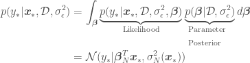
 ,
,  being the independent variables and
  the dependent variable,
  is a vector of model parameters and
  is the model error variance. The unusual notation for the normal distribution
  means “a normal distribution of
  and variance
  ,” where
  is the number of points in the data set. The estimated variance of
  ,
,  can be calculated as
 and
and  are the mean and the covariance of the
  with an error variance of
  ), replace
  and
and  , e.g.
  , to add features to
  , we would instead have that

 and
and  . One problem with this approach is that as we add more terms (also called features) to function
  to better capture non-linearities, the the dimension of the matrix we will have to invert increases. It is also not always obvious what features we should add to our data. Both problems can be handled with Gaussian Processes.
 we have to invert (remember the dimensions of such matrix equals the number of features in

 —
—  is just another point
  either in the data set or for which we want to estimate
  will be called a covariance or kernel function. Since the prior’s covariance
 . Using
  and assuming a prior of
  ,
, 

 ,
,  and
and  . Now the features of the data are absorbed within the inner-products between observed
  ‘s and or for
  , is that
  does not have to represent simply a matrix-matrix or vector-matrix multiplication of
  , which will necessarily return a positive semi-definite matrix and therefore be a valid covariance matrix. There are several kernels (or kernel functions or kernel shapes) available, each accounting in a different way for the nearness or similarity (at least in Gaussian Processes) between values of
  :
: . This kernel is used when trying to fit a line going through the origin.
 , where d is the dimension of the polynomial function. This kernel is used when trying to fit a polynomial function (such as the fourth order polynomial in the blog post about Bayesian OLR), and
 , where
  is a kernel parameter denoting the characteristic length scale of the function to be approximated. Using the RBF kernel is equivalent to adding an infinite (!) number of features the data, meaning
  .
. at discrete points, with a collection of
  for all
  . After all, don’t we want a function more often than not solely for the purpose of getting point estimates and associated errors for given values of
  . The mean of all possible functions at
  in
in  will be for each pair
  based on the value of a distance metric between
  tend to be similar and vice-versa. We can therefore turn the sampled functions
  into whatever functional form we want by choosing the appropriate covariance matrix (kernel) — e.g. a linear kernel will return a linear model, a polynomial kernel will return a polynomial function, and an RBF kernel will return a function with an all linear and an infinite number of non-linear terms. A Gaussian Process can then be written as
 is the mean function (e.g. a horizontal line along the x-axis at y = 0 would mean that
 ![\mu(\boldsymbol{x}) = [0,..,0]^T](https://s0.wp.com/latex.php?latex=%5Cmu%28%5Cboldsymbol%7Bx%7D%29+%3D+%5B0%2C..%2C0%5D%5ET&bg=ffffff&fg=444444&s=0&c=20201002) ) and
) and  along the x-axis from x=-5 to x=5 (
 ) using a Gaussian Process. Assume the parameters of our Gaussian Process from which we will sample our functions are mean 0 and that it uses an RBF kernel for its covariance matrix with parameter
  (not be confused with standard deviation), meaning that
 ![k_{i,i}=1.0 ,\:\forall i \in [0, 199]](https://s0.wp.com/latex.php?latex=k_%7Bi%2Ci%7D%3D1.0+%2C%5C%3A%5Cforall+i+%5Cin+%5B0%2C+199%5D&bg=ffffff&fg=444444&s=0&c=20201002) and
and ![k_{i,j}=e^{-\frac{||x_i-x_j||^2}{2\cdot 2^2}},\: \forall i,j \in [0, 199]](https://s0.wp.com/latex.php?latex=k_%7Bi%2Cj%7D%3De%5E%7B-%5Cfrac%7B%7C%7Cx_i-x_j%7C%7C%5E2%7D%7B2%5Ccdot+2%5E2%7D%7D%2C%5C%3A+%5Cforall+i%2Cj+%5Cin+%5B0%2C+199%5D&bg=ffffff&fg=444444&s=0&c=20201002) , or
, or![\begin{aligned} p(\boldsymbol{f}_*|\boldsymbol{X_*})&=\mathcal{N}(\boldsymbol{f}|\boldsymbol{\mu},\boldsymbol{K_{**}})\\ &=\mathcal{N}\left(\boldsymbol{f}_*\Bigg|[\mu_{*0},..,\mu_{*199}], \begin{bmatrix} k_{*0,0} & k_{*0,1} & \cdots & k_{*0,199} \\ k_{*1,0} & k_{*1, 1} & \cdots & k_{*1,199}\\ \vdots & \vdots & \ddots & \vdots \\ k_{*199,0} & k_{*199,1} & \cdots & k_{*199,199} \end{bmatrix} \right)\\ &=\mathcal{N}\left(\boldsymbol{f}_*\Bigg|[0,..,0], \begin{bmatrix} 1 & 0.9997 & \cdots & 4.2\cdot 10^{-6} \\ 0.9997 & 1 & \cdots & 4.8\cdot 10^{-6}\\ \vdots & \vdots & \ddots & \vdots \\ 4.2\cdot 10^{-6} & 4.8\cdot 10^{-6} & \cdots & 1 \end{bmatrix} \right) \end{aligned}](https://s0.wp.com/latex.php?latex=%5Cbegin%7Baligned%7D+p%28%5Cboldsymbol%7Bf%7D_%2A%7C%5Cboldsymbol%7BX_%2A%7D%29%26%3D%5Cmathcal%7BN%7D%28%5Cboldsymbol%7Bf%7D%7C%5Cboldsymbol%7B%5Cmu%7D%2C%5Cboldsymbol%7BK_%7B%2A%2A%7D%7D%29%5C%5C+%26%3D%5Cmathcal%7BN%7D%5Cleft%28%5Cboldsymbol%7Bf%7D_%2A%5CBigg%7C%5B%5Cmu_%7B%2A0%7D%2C..%2C%5Cmu_%7B%2A199%7D%5D%2C+%5Cbegin%7Bbmatrix%7D+k_%7B%2A0%2C0%7D+%26+k_%7B%2A0%2C1%7D+%26+%5Ccdots+%26+k_%7B%2A0%2C199%7D+%5C%5C+k_%7B%2A1%2C0%7D+%26+k_%7B%2A1%2C+1%7D+%26+%5Ccdots+%26+k_%7B%2A1%2C199%7D%5C%5C+%5Cvdots+%26+%5Cvdots+%26+%5Cddots+%26+%5Cvdots+%5C%5C+k_%7B%2A199%2C0%7D+%26+k_%7B%2A199%2C1%7D+%26+%5Ccdots+%26+k_%7B%2A199%2C199%7D+%5Cend%7Bbmatrix%7D+%5Cright%29%5C%5C+%26%3D%5Cmathcal%7BN%7D%5Cleft%28%5Cboldsymbol%7Bf%7D_%2A%5CBigg%7C%5B0%2C..%2C0%5D%2C+%5Cbegin%7Bbmatrix%7D+1+%26+0.9997+%26+%5Ccdots+%26+4.2%5Ccdot+10%5E%7B-6%7D+%5C%5C+0.9997+%26+1+%26+%5Ccdots+%26+4.8%5Ccdot+10%5E%7B-6%7D%5C%5C+%5Cvdots+%26+%5Cvdots+%26+%5Cddots+%26+%5Cvdots+%5C%5C+4.2%5Ccdot+10%5E%7B-6%7D%C2%A0%26%C2%A04.8%5Ccdot+10%5E%7B-6%7D+%26+%5Ccdots+%26+1+%5Cend%7Bbmatrix%7D+%5Cright%29+%5Cend%7Baligned%7D&bg=ffffff&fg=444444&s=0&c=20201002)
![\boldsymbol{f}_* = [y_0, ..., y_{199}]](https://s0.wp.com/latex.php?latex=%5Cboldsymbol%7Bf%7D_%2A+%3D+%5By_0%2C+...%2C+y_%7B199%7D%5D&bg=ffffff&fg=444444&s=0&c=20201002) . A draw of 3 such sample functions would look generally like the following:
. A draw of 3 such sample functions would look generally like the following:
 . All we have to do is to add random variables corresponding to our data and condition the resulting distribution on them, which means accounting only for samples of functions that exactly go through (or given) our data points. The resulting distribution would then look like
  . After adding our data
  , or
, or  , our distribution would look like
 from which we want to get point estimates and corresponding error standard deviations. The covariance matrix above accounts for correlations of all observations with all other observations, and correlations of all observations with all points to be predicted. We now just have to


 ,
,  ,
,  , and
, and  is a vector containing the elements in the diagonal of the covariance matrix
  — the variances
  of each random variable
 ![\boldsymbol{\mu} = \boldsymbol{\mu}_* = [0, ... , 0]^T](https://s0.wp.com/latex.php?latex=%5Cboldsymbol%7B%5Cmu%7D+%3D+%5Cboldsymbol%7B%5Cmu%7D_%2A+%3D+%5B0%2C+...+%2C+0%5D%5ET&bg=ffffff&fg=444444&s=0&c=20201002) , the mean of the Gaussian Process would be
, the mean of the Gaussian Process would be  . A plot of
  estimated for 200 values of
  ), regressed on 5 random data points
 should look generally like
 of the RBF kernel, which determines the correlation length scale of the fitted model and therefore how fast with increasing separation distance between data points the model will default to the prior (here, with
  ). The figure below exemplifies this effect


 , we’d do something like:
 and variance
  for each of the regression model parameters
 is defined as
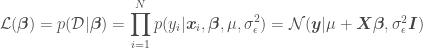
 is the mean of the model error (normally
  ),
),  . Digression: in Generalized Linear Regression (GLR), observations may not be independent and may have different variances (heteroscedasticity), so the covariance matrix may have off-diagonal terms and the diagonal terms may not be equal.
 for this function, but do not confuse it with a normal distribution. This procedure is called basis function expansion and has a likelihood function of the form

 , called the parameter posterior distribution, is calculated by multiplying the likelihood function used in MLE by a prior distribution for the parameters. A prior distribution is assumed from knowledge prior to analyzing new data. In Bayesian Linear Regression, a Gaussian distribution is commonly assumed for the parameters. For example, the prior on
  for algebraic simplicity. The parameter posterior distribution assuming a known
  , given
  is a constant depending only on the data.

 for a data set
  for data set
 , with
  denoting a new point that is not in
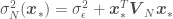


![\phi(x) = [1, x, x^2, x^3, x^4]^T](https://s0.wp.com/latex.php?latex=%5Cphi%28x%29+%3D+%5B1%2C+x%2C+x%5E2%2C+x%5E3%2C+x%5E4%5D%5ET&bg=ffffff&fg=444444&s=0&c=20201002) and the resulting
and the resulting  would therefore have five columns instead of two (
![[1, x]^T](https://s0.wp.com/latex.php?latex=%5B1%2C+x%5D%5ET&bg=ffffff&fg=444444&s=0&c=20201002) ), so now the task is to find
), so now the task is to find ![\boldsymbol{\beta}=[\beta_0, \beta_1, \beta_2, \beta_3, \beta_4]^T](https://s0.wp.com/latex.php?latex=%5Cboldsymbol%7B%5Cbeta%7D%3D%5B%5Cbeta_0%2C+%5Cbeta_1%2C+%5Cbeta_2%2C+%5Cbeta_3%2C+%5Cbeta_4%5D%5ET&bg=ffffff&fg=444444&s=0&c=20201002) . Following the same logic as before for
. Following the same logic as before for  and
and  , where prime denotes the new set random variable
  from function

