Introduction to Gaussian Processes

In this post, I will cover the very basics of Gaussian Processes following the presentations in Murphy (2012) and Rasmussen and Williams (2006) — though hopefully easier to digest. I will approach the explanation in two ways: (1) derived from Bayesian Ordinary Linear Regression and (2) derived from the definition of Gaussian Processes in functional space (it is easier than it sounds). I am not sure why the mentioned books do not use “^” to denote estimation (if you do, please leave a comment), but I will stick to their notation assuming you may want to look into them despite running into the possibility of an statistical sin. Lastly, I would like to thank Jared Smith for reviewing this post and providing highly statistically significant insights.

If you are not familiar with Bayesian regression (see my previous post), skip the section below and begin reading from “Succinct derivation of Gaussian Processes from functional space.”

From Bayesian Ordinary Linear Regression to Gaussian Processes

Recapitulation of Bayesian Ordinary Regression

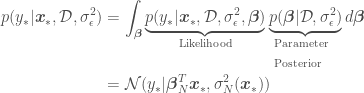
In my previous blog post, about Bayesian Ordinary Linear Regression (OLR), I showed that the predictive distribution for a point for which we are trying to estimate with Bayesian OLR is

where we are trying to regress a model over the data set , being the independent variables and the dependent variable, is a vector of model parameters and is the model error variance. The unusual notation for the normal distribution means “a normal distribution of with (or given) the regression mean and variance ,” where is the number of points in the data set. The estimated variance of , and the estimated regression parameters can be calculated as

where and are the mean and the covariance of the parameter prior distribution. All the above can be used to estimate as

with an error variance of

If we assume a prior mean of 0 (), replace and by their definitions, and apply a function , e.g. , to add features to so that we can use a linear regression approach to fit a non-linear model over our data set , we would instead have that

where and . One problem with this approach is that as we add more terms (also called features) to function  to better capture non-linearities, the the dimension of the matrix we will have to invert increases. It is also not always obvious what features we should add to our data. Both problems can be handled with Gaussian Processes.

Now to Gaussian Processes

This is where we transition from Bayesian OLR to Gaussian Processes. What we want to accomplish in the rest of this derivation is to find a way of: (1) adding as many features to the data as we need to calculate  and without increasing the size of the matrix we have to invert (remember the dimensions of such matrix equals the number of features in ), and of (2) finding a way of implicitly adding features to  and without having to do so manually — manually adding features to the data may take a long time, specially if we decide to add (literally) an infinite number of them to have an interpolator.

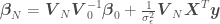
The first step is to make the dimensions of the matrix we want to invert equal to the number of data points instead of the number of features in . For this, we can re-arrange the equations for and as

We now have our feature-expanded data and points for which we want point estimates always appearing in the form of — is just another point either in the data set or for which we want to estimate . From now on, will be called a covariance or kernel function. Since the prior’s covariance is positive semi-definite (as any covariance matrix), we can write

where . Using and assuming a prior of , and then take a new shape in the predictor posterior of a Gaussian Process:

where , and . Now the features of the data are absorbed within the inner-products between observed ‘s and or for , so we can add as many features as we want without impacting the dimensions of the matrix we will have to invert. Also, after this transformation, instead of and representing the mean and covariance between model parameters, they represent the mean and covariance of and among data points and/or points for which we want to get point estimates. The parameter posterior from Bayesian OLR would now be used to sample the values of directly instead of model parameters. And now we have a Gaussian Process with which to estimate . For plots of samples of from the prior and from the predictive posterior, of the mean plus or minus the error variances, and of models with different kernel parameters, see figures at the end of the post.

Kernel (or Covariance) matrices

The convenience of having and written in terms of , is that does not have to represent simply a matrix-matrix or vector-matrix multiplication of and . In fact, function can be any function that corresponds to an inner-product after some transformation from , which will necessarily return a positive semi-definite matrix and therefore be a valid covariance matrix. There are several kernels (or kernel functions or kernel shapes) available, each accounting in a different way for the nearness or similarity (at least in Gaussian Processes) between values of :

• the linear kernel: . This kernel is used when trying to fit a line going through the origin.
• the polynomial kernel: , where d is the dimension of the polynomial function. This kernel is used when trying to fit a polynomial function (such as the fourth order polynomial in the blog post about Bayesian OLR), and
• the Radial Basis Function, or RBF (aka Squared Exponential, or SE), 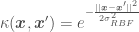, where is a kernel parameter denoting the characteristic length scale of the function to be approximated. Using the RBF kernel is equivalent to adding an infinite (!) number of features the data, meaning .

But this is all quite algebraic. Luckily, there is a more straight-forward derivation shown next.

Succinct derivation of Gaussian Processes from functional space.

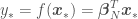
Most regression we study in school is a way of estimating the parameters of a model. In Bayesian OLR, for example, we have a distribution (the parameter posterior) from which to sample model parameters. What if we instead derived a distribution from which to sample functions themselves? The first (and second and third) time I heard about the idea of sampling functions I thought right away of opening a box and from it drawing exponential and sinusoid functional forms. However, what is meant here is a function of an arbitrary shape without functional form. How is this possible? The answer is: instead of sampling a functional form itself, we sample the values of at discrete points, with a collection of for all in our domain called a function . After all, don’t we want a function more often than not solely for the purpose of getting point estimates and associated errors for given values of ?

In Gaussian Process regression, we sample functions  from a distribution by considering each value of in a discretized range along the x-axis as a random variable. That means that if we discretize our x-axis range into 100 equally spaced points, we will have 100 random variables . The mean of all possible functions at therefore represents the mean value of in , and each term in the covariance matrix (kernel matrix, see “Kernel (or Covariance) matrices” section above) represents how similar the values of and  will be for each pair and  based on the value of a distance metric between  and : if and  are close to each other, and  tend to be similar and vice-versa. We can therefore turn the sampled functions into whatever functional form we want by choosing the appropriate covariance matrix (kernel) — e.g. a linear kernel will return a linear model, a polynomial kernel will return a polynomial function, and an RBF kernel will return a function with an all linear and an infinite number of non-linear terms. A Gaussian Process can then be written as

where is the mean function (e.g. a horizontal line along the x-axis at y = 0 would mean that ) and is the covariance matrix, which here expresses how similar the values of will be based on the distance between two values of .

To illustrate this point, assume we want to sample functions over 200 discretizations along the x-axis from x=-5 to x=5 () using a Gaussian Process. Assume the parameters of our Gaussian Process from which we will sample our functions are mean 0 and that it uses an RBF kernel for its covariance matrix with parameter (not be confused with standard deviation), meaning that and , or

Each sample from the normal distribution above will return 200 values: . A draw of 3 such sample functions would look generally like the following:

The functions above look incredibly smooth because of the RBF kernel, which adds an infinite number of non-linear features to the data. The shaded region represents the prior distribution of functions. The grey line in the middle represents the mean of an infinite number of function samples, while the upper and lower bounds represent the corresponding prior mean plus or minus standard deviations.

These functions looks quite nice but pretty useless. We are actually interested in regressing our data assuming a prior, namely on a posterior distribution, not on the prior by itself. Another way of formulating this is to say that we are interested only in the functions that go through or close to certain known values of and . All we have to do is to add random variables corresponding to our data and condition the resulting distribution on them, which means accounting only for samples of functions that exactly go through (or given) our data points. The resulting distribution would then look like . After adding our data , or , our distribution would look like

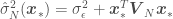
In this distribution we have random variables representing the from our data set and the  from which we want to get point estimates and corresponding error standard deviations. The covariance matrix above accounts for correlations of all observations with all other observations, and correlations of all observations with all points to be predicted. We now just have to condition the multivariate normal distribution above over the points in our data set, so that the distribution accounts for the infinite number of functions that go through our at the corresponding . This yields

where , , , and is a vector containing the elements in the diagonal of the covariance matrix — the variances of each random variable . If you do not want to use a prior with , the mean of the Gaussian Process would be . A plot of estimated for 200 values of — so that the resulting curve looks smooth — plus or minus associated uncertainty (), regressed on 5 random data points , , should look generally like

 

A plot of three sampled functions (colored lines below, the grey line is the mean) should look generally like

 

Several kernel have parameters that can strongly influence the regressed model and that can be estimated — see Murphy (2012) for a succinct introduction to kernel parameters estimation. One example is parameter of the RBF kernel, which determines the correlation length scale of the fitted model and therefore how fast with increasing separation distance between data points the model will default to the prior (here, with ). The figure below exemplifies this effect

All figures have the same data points but the resulting models look very different. Reasonable values for depend on the spacing between the data points and are therefore data-specific. Also, if when you saw this plot you thought of fitting RBF functions as interpolators, that was not a coincidence: the equations solved when fitting RBFs to data as interpolators are the same solved when using Gaussian Processes with RBF kernels.

Lastly, in case of noisy observation of in the Gaussian Process distribution and the expressions for the mean, covariance, and standard deviation become

where is the error variance and is an identity matrix. The mean and error predictions would look like the following

Concluding Remarks

What I presented is the very basics of Gaussian Processes, leaving several important topics which were not covered here for the interested reader to look into. Examples are numerically more stable formulations, computationally more efficient formulations, kernel parameter estimation, more kernels, using a linear instead of zero-mean prior (semi-parametric Gaussian Processes), Gaussian Processes for classification and Poisson regression, the connection between Gaussian Processes and other methods, like krieging and kernel methods for nonstationary stochastic processes. Some of these can be found in great detail in Rasmussen and Williams (2006), and Murphy (2012) has a succinct presentation of all of the listed topics.

I was really confused about Gaussian Processes the first time I studied it and tried to make this blog post as accessible as possible. Please leave a comment if you think the post would benefit from any particular clarification.

 

References

Murphy, Kevin P., 2012. Machine Learning: A Probabilistic Perspective. The MIT Press, ISBN 978-0262018029

Rasmussen, Carl Edward and Williams, Christopher K. I., 2006. Gaussian Processes for Machine Learning. The MIT Press, ISBN 978-0262182539.