
This post was inspired by the Sankey diagram in Figure 1 of this pre-print led by Dave Gold: “Exploring the Spatially Compounding Multi-sectoral Drought Vulnerabilities in Colorado’s West Slope River Basins” (Gold, Reed & Gupta, In Review) which features a Sankey diagram of flow contributions to Lake Powell. I like the figure, and thought I’d make an effort to produce similar diagrams using USGS gauge data.
Sankey diagrams show data flows between different source and target destinations. Lot’s of people use them to visualize their personal/business cashflows. It’s an obvious visualization option for streamflows.
To explain the “(?)” in my title: When I started this, I’d realized quickly that I to choose one of two popular plotting packages: matplotlib or plotly.
I am a frequent matplotlib user and definitely appreciate the level of control in the figure generation process. However, it can sometimes be more time- and line-intensive designing highly customized figures using matplotlib. On the other hand, in my experience, plotly tools can often produce appealing graphics with less code. I am also drawn to the fact that the plotly graphics are interactive objects rather than static figures.
I decided to go with plotly to try something new. If you want to hear my complaints and thoughts on use context, you can skip to the conclusions below.
In the sections below, I provide some code which will:
- Define a network of USGS gauge stations to include in the plot
- Retrieve data from USGS gauge stations
- Create a Sankey diagram using plotly showing streamflows across the network
Here, I focus on the Rio Grande river upstream of Albuquerque, NM. However you can plot a different streamflow network by modifying the dictionary of upstream nodes defining the network.
Plotting a Sankey streamflow network with plotly
The code used here requires both plotly and the pygeohydro package (for USGS data retrieval).
from pygeohydro import NWIS
import plotly.graph_objects as go
With that out of the way, we can get started.
Defining the flow network & data retrieval
I start by defining a dictionary called upstream_stations which defines the relationships between different gauges of interest.
This dictionary contains pairs of the form:
{"GAUGE_ID" : ["LIST_OF", "UPSTREAM", "GAUGE_IDs"]}
If there is no upstream site, then include an empty list. For the Rio Grande network, this looks like:
# define relationships between each gauge and upstream sites
upstream_stations = {
    '08329918' : ['08319000', '08328950'],
    '08319000' : ['08317400', '08317200'],
    '08328950' : [],
    '08317200' : [],
    '08317400' : ['08313000'],
    '08313000' : ['08290000', '08279500'],
    '08287000' : [],
    '08279500' : [],
    '08290000' : ['08287000', '08289000'],
    '08289000' : [],
}

# Get list of all stations from upstream_stations
all_stations = list(upstream_stations.keys())
for station, upstream in upstream_stations.items():
    all_stations += upstream
all_stations = list(set(all_stations))
Notice that I also made a list containing all the stations IDs. I use the pygeohydro package from the HyRiver suite of tools to get retrieve the gauge station data (Chegini, Li, & Leung, 2021). I often cite this package, and have written about it in a past post (“Efficient hydroclimatic data accessing with HyRiver for Python”).
Using the list of all_stations, I use the following code to pull daily streamflow data for each site from 2015-2020 (or some other specified dates):
def get_usgs_gauge_data(stations, dates):
    """
    Get streamflow data from USGS gauge stations using NWIS.
    """
    nwis = NWIS()
    df = nwis.get_streamflow(stations, dates, mmd=False)

    # get rid of USGS- in columns
    df.columns = df.columns.str.replace('USGS-', '')
    return df

# Get USGS flows
flows = get_usgs_gauge_data(all_stations, ('2015-01-01', '2020-12-31'))
For the Sankey diagram, we need a single flow value for each station. In this case I calculate an average of the annual total flows at each station:
# Get annual mean flows
agg_flows = flows.resample('Y').sum().agg('mean')
Creating the Sankey figure
At it’s core, a Sankey diagram is a visualization of a weighted network (also referred to as a graph) defined by:
- Nodes
- Links (aka Edges)
- Weights
In our case, the nodes are the USGS gauge stations, the links are the connections between upstream and downstream gauges, and the weights are the average volumes of water flowing from one gauge to the next.
Each link is defined by a source and target node and a value. This is where the upstream_stations dictionary comes in. In the code block below, I set up the nodes and links, looping through upstream_stations to define all of the source-target relationships:
## Deinfe nodes and links
# Nodes are station IDs
nodes = all_stations
node_indices = {node: i for i, node in enumerate(nodes)}

# make links based on upstream-downstream relationships
links = {
    'source': [],
    'target': [],
    'value': [],
}

# loop through upstream_stations dict
for station, upstream_list in upstream_stations.items():
    for stn in upstream_list:
        if stn in agg_flows and station in agg_flows:
            links['source'].append(node_indices[stn])
            links['target'].append(node_indices[station])
            links['value'].append(agg_flows[stn])
Lastly, I define some node labels and assign colors to each node. In this case, I want to make the nodes black if they represent reservoir releases (gauges at reservoir outlets) or blue if they are simple gauge stations.
labels = {
    '08329918' : 'Rio Grande at Alameda',
    '08319000' : 'San Felipe Gauge',
    '08328950' : 'Jemez Canyon Reservoir',
    '08317200' : 'Santa Fe River',
    '08317400' : 'Cochiti Reservoir',
    '08313000' : 'Rio Grande at Otowi Bridge',
    '08287000' : 'Abiquiu Reservoir',
    '08279500' : 'Rio Grande',
    '08290000' : 'Rio Chama',
    '08289000' : 'Rio Ojo Caliente',
}

# Create nodes labels and colors lists
node_labels = [labels[node] for node in nodes]
node_colors = ['black' if 'Reservoir' in label else 'dodgerblue' for label in node_labels]
Finally, the function to generate the figure:
def create_sankey_diagram(node_labels, links, node_colors,
						  orientation='h',
                          size=(2000, 700)):
    """
    Create a Sankey diagram of using Plotly.

    Parameters
    ----------
    node_labels : list
        List of node labels.
    links : dict
        Dictionary with keys 'source', 'target', and 'value'.
    node_colors : list
        List of node colors.
    orientation : str
        Orientation of the diagram, 'h' for horizontal and 'v' for vertical.

    Returns
    -------
    sankey_fig : plotly.graph_objects.Figure
        Plotly figure object.
    """
    sankey_fig = go.Figure(go.Sankey(
        orientation=orientation,
        node=dict(
            pad=70,
            thickness=45,
            line=dict(color='dodgerblue', width=0.5),
            label=node_labels,
            color=node_colors
        ),
        link=dict(
            source=links['source'],
            target=links['target'],
            value=links['value'],
            color='cornflowerblue'
        )
    ))

    sankey_fig.update_layout(
        title_text="Rio Grande Streamflow ",
        font=dict(size=23),
        width=size[0],
        height=size[1]
    )
    return sankey_fig
There are some options for manipulating this figure script to better suit your needs. Specifically you may want to modify:
pad=70: this is the horizontal spacing between nodesthickness=45: this is the thickness of the node elements
With our pre-prepped data from above, we can use the function like so:
sankey_fig = create_sankey_diagram(node_labels,
								   links,
								   node_colors,
								   orientation='v', size=(1000, 1200))
sankey_fig
And here we have it:

I’d say it looks… okay. And admittedly this is the appearance after manipulating the node placement using the interactive interface.
It’s a squished vertically (which can be improved by making it a much taller figure). However my biggest issue is with the text being difficult to read.
Changing the orientation to horizontal (orientation='h') results in a slightly better looking figure. Which makes sense, since the Sankey diagram is often shown horizontal. However, this does not preserve the relationship to the actual North-South flow direction in the Rio Grande, so I don’t like it as much.

Conclusions
To answer the question posed by the title, “Sankey diagrams for USGS gauge data in python(?)”: Yes, sometimes. And sometimes something else.
Plotly complaints: While working on this post, I developed a few complaints with the plotly Sankey tools. Specifically:
- It appears that the label text coloring cannot be modified. I don’t like the white edgecolor/blur effect, but could not get rid of this.
- The font is very difficult to read… I had to make the text size very large for it to be reasonably legible.
- You can only assign a single node thickness. I had wanted to make the reservoirs thick, and shrink the size of the gauge station nodes. However, it seems this cannot be done.
- The diagrams appear low-resolution and I don’t see a way to save a high res version.
Ultimately, the plotly tools are very restrictive in the design of the graphic. However, this is a tradeoff in order to get the benefit of interactive graphics.
Plotly praise: The plotly Sankey tools have some advantages, specifically:
- The plots are interactive
- Plots can be saved as HTML and embedded in websites
These advantages make the plotly tools good for anyone who might want to have a dynamic and maybe frequently updated dashboard on a site.
On the other hand, if I wanted to prepare a publication-quality figure, where I had absolute control of the design elements, I’d likely turn to matplotlib. That way it could be saved as an SVG and further manipulated in a vector art program link Inkscape or Illustrator.
Thanks for reading!
References
Chegini, T., Li, H. Y., & Leung, L. R. (2021). HyRiver: Hydroclimate data retriever. Journal of Open Source Software, 6(66), 3175.
Links
- Matplotlib Sankey documentation
- Plotly Sankey plotting documentation
- A website by author Phineas housing 82 pages of Sankey diagram examples: https://www.sankey-diagrams.com/
- The pySankey package by anazalea on github which uses matplotlib but appears to no longer be maintained


")

 The Good:


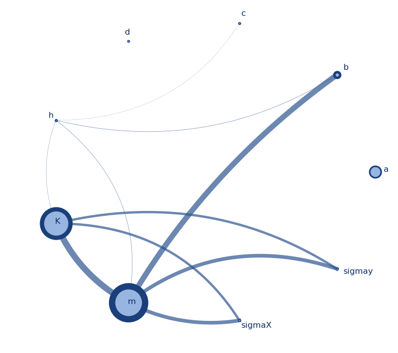
 Curvatures


