Efficient hydroclimatic data accessing with HyRiver for Python

This tutorial highlights the HyRiver software stack for Python, which is a very powerful tool for acquiring large sets of data from various web services.

I have uploaded a Jupyter-Notebook version of this post here if you would like to execute it yourself.

HyRiver Introduction

The HyRiver software suite was developed by Taher Chegini who, in their own words, describes HyRiver as:

“… a software stack consisting of seven Python libraries that are designed to aid in hydroclimate analysis through web services.”

This description does not do justice to the capability of this software. Through my research I have spent significant amounts of time wrangling various datasets – making sure that dates align, or accounting for spatial misalignment of available data. The HyRiver suite streamlines this process, and makes acquisition of different data from various sources much more efficient.

Here, I am going walk through a demonstration of how to easily access large amounts of data (streamflow, geophysical, and meteorological) for a basin of interest.

Before going through the code, I will highlight the three libraries from the HyRiver stack which I have found most useful: PyGeoHydro, PyNHD, and PyDaymet.

PyGeohydro

PyGeoHydro allows for interaction with eight different online datasets, including:

• USGS National Water Information System (NWIS)
• NCAR Catchment Attributes and Meteorology for Large-sample Studies (CAMELS)
• USGS Water Quality Portal
• US ACE National Invetory of Dams (NID)

In this tutorial, I will only be interacting with the USGS NWIS, which provides daily streamflow data.

PyNHD

The PyNHD library is designed to interact with the National Hydrography Dataset (NHD)and the Hydro Network-Linked Data Index (NLDI).

NHDPlus (National Hydrography Dataset)

The NHD defines a high-resolutioon network of stream linkages, each with a unique idenfier (ComID).

NLDI (Network-Linked Data Index)

The NLDI aids in the discovery of indexed information along some NHD-specified geometry (ComIDs). The NLDI essentially tranverses the linkages specified by the NHD geometry and generates data either local or basin-aggregated data relative to a specific linkage (ComID).

As will be seen later in the tutorial, the NLDI is able to retrieve at least 126 different types of data for a given basin…

PyDaymet

The PyDaymet GirHub repository summarizes the package as:

“[providing] access to climate data from Daymet V4 database using NetCDF Subset Service (NCSS). Both single pixel (using get_bycoords function) and gridded data (using get_bygeom) are supported which are returned as pandas.DataFrame and xarray.Dataset, respectively.”

Tutorial outline:

0. Installation
1. Retrieving USGS Water Data
2. Retrieving Geophysical (NLDI) Data
3. Retrieving Daymet Data

The HyRiver repository contains various examples demonstrating the use of the various libraries. I would definitely recommend digging in deeper to these, and other HyRiver documentation if this post piques your interest.

Step 0: Installation

In this tutorial, I only only interact with the PyNHD, PyGeoHydro, and PyDaymet libraries, so I do not need to install all of the HyRiver suite.

If you operate through pip, you can install these libraries using:

pip install pynhd pygeohydro pydaymet

If you use Anaconda package manager, you can install these packages using:

conda install -c conda-forge pynhd pygeohydro pydaymet

For more information on installation, refer to the HyRiver GitHub repository and related documentation.

Now, onto the fun part!

Step 1: Retreiving USGS Water Data

I am beginning here because streamflow data is typically the first point of interest for most hydrologic engineers or modelers.

Personally, I have gone through the process of trying to download data manually from the USGS NWIS website… My appreciation for the USGS prevents me from saying anything too negative, but let’s just say it was not a pleasant experience.

Pygeohydro allows for direct requests from the USGS National Water Information System (NWIS), which provides daily streamflow data from all USGS gages. The data is conveniently output as a Pandas DataFrame.

With this functionality alone, the PyGeoHydro library is worth learning.

1.1 Initialize PyGeoHydro NWIS tool

# Import common libraries
import numpy as np
import pandas as pd
import matplotlib.pyplot as plt

# Import the PyGeohydro libaray tools
import pygeohydro as gh
from pygeohydro import NWIS, plot

# Use the national water info system (NWIS)
nwis = NWIS()

1.2 Requesting USGS Streamflow Data

The get_streamflow() function does exactly as the name entails and will retrieve daily streamflow timeseries, however USGS gage station IDs must be provided. If you are only interested in a single location, then you can enter 8-digit gage ID number along with a specified date range to generate the data:

get_streamflow('########', dates = ('Y-M-D', 'Y-M-D'))

However, I am want to explore larger sets of data over an entire region. Thus, I am going to use PyGeoHydro's get_info() function to identify all gages within some region of interest.

First, I specify a region via (latitude, longitude) bounds, then I send a query which retrieves meta-data information on all the gages in the specified region. In this case, I am exploring the data available near Ithaca, NY.

# Query specifications
region = (-76.7, 42.3, -76, 42.6) # Ithaca, NY

# Send a query for all gage info in the region
query = {"bBox": ",".join(f"{b:.06f}" for b in region),
         "hasDataTypeCd": "dv",
         "outputDataTypeCd": "dv"}

info_box = nwis.get_info(query)

print(f'PyGeoHydro found {len(set(info_box.site_no))} unique gages in this region.')

# [Out]: PyGeoHydro found #N unique gages in this region.

Although, this info_box identify many gages in the region which have very old or very brief data records. Knowing this, I want to filter out data which does not have a suitable record length.

For the sake of this tutorial, I am considering data between January 1st, 2020 and December 31st, 2020.

# Specify date range of interest
dates = ("2020-01-01", "2020-12-31") 

# Filter stations to have only those with proper dates
stations = info_box[(info_box.begin_date <= dates[0]) & (info_box.end_date >= dates[1])].site_no.tolist()

# Remove duplicates by converting to a set
stations = set(stations)

Now, I am ready to use the gage IDs contained in stations to request the streamflow data!

# Retrieve the flow data
flow_data = nwis.get_streamflow(stations, dates, mmd=False)

# Remove gages with nans
flow_data = flow_data.dropna(axis = 1, how = 'any')

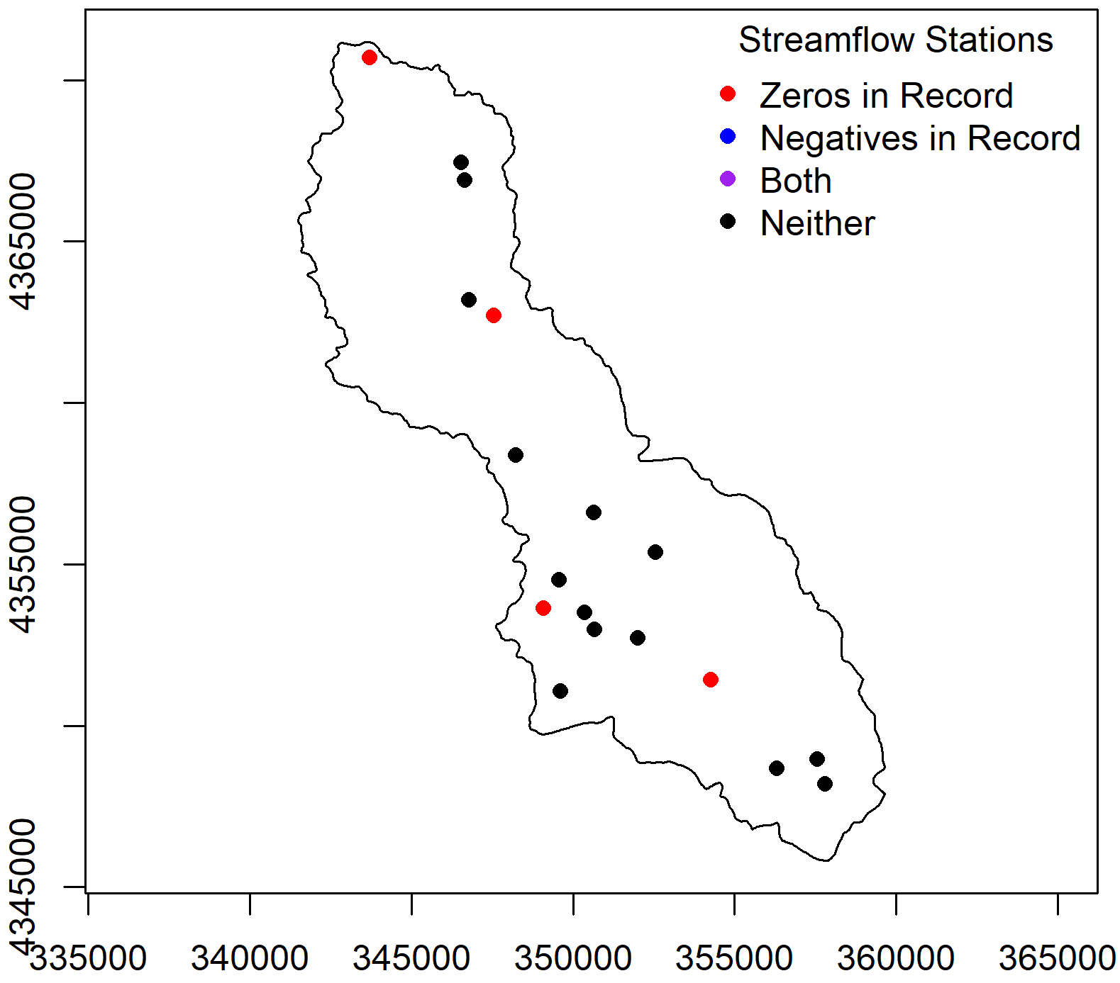
After removing duplicates and gages with nans, I have data from five unique gages in this region.

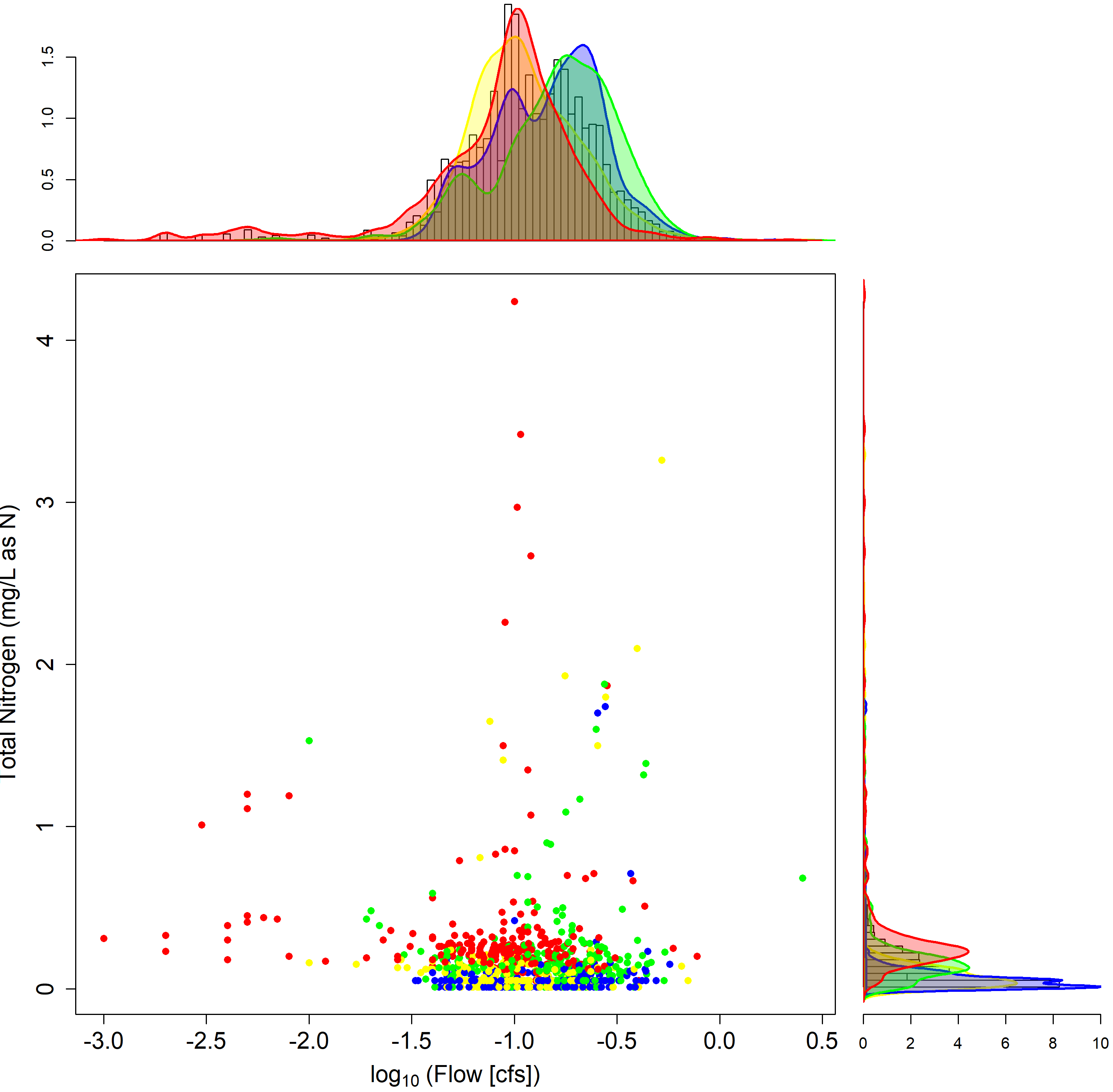
Additionally, PyGeoHydro has a convenient plotting feature to help quickly visualize the streamflow data.

from pygeohydro import plot

# Plot flow data summary
plot.signatures(flow_data)

Summary of flow data for the 5 gages found with PyGeoHydro.

There is a lot more to be explored in the PyGeoHydro library, but I will leave that up to the curious reader.

Step 2: Retrieving Geophysical (NLDI) Data

So, you’ve got some streamflow data but you don’t know anything about the physical watershed…

This is where the PyNHD library comes in. Using this library, I can identify entire upstream network from a gage, then extract the NLDI data associated with the watershed linkages.

# Import the PyNHD library
import pynhd as pynhd
from pynhd import NHD
from pynhd import NLDI, WaterData

First, we can take a look at all possible local basin characteristic data that are available:

# Get list of local data types (AKA characteristics, or attributes)
possible_attributes = NLDI().get_validchars("local").index.to_list()

There are 126 characteristics available from the NLDI! These characteristics range from elevation, to reservoir capacity, to bedrock depth. Many if these are not of immediate interest to me, so I will specify a subset of select_attributes to retrieve (basin area, max elevation, and stream slope).

I then loop through all of my USGS stations for which I have data in flow_data, identifying the upstream basin linkages using NLDI().navigate_byid(). Once the basin is identified, I extract the ComID numbers for each linkage and use that number to retrieve the NLDI data of interest. I then store the data in nldi_data. This process is done by the following:

# Specify characteristics of interest
select_attributes = ['CAT_BASIN_AREA', 'CAT_ELEV_MAX', 'CAT_STREAM_SLOPE']

# Initialize a storage matrix
nldi_data = np.zeros((len(flow_data.columns), len(select_attributes)))

# Loop through all gages, and request NLDI data near each gage
for i, st in enumerate(flow_data.columns):

    # Navigate up all flowlines from gage
    flowlines = NLDI().navigate_byid(fsource = 'nwissite',
                                    fid = f'{st}',
                                    navigation="upstreamTributaries",
                                    source = 'flowlines',
                                    distance = 10)

    # Get the nearest comid
    station_comid = flowlines.nhdplus_comid.to_list()[0]

    # Source NLDI local data
    nldi_data[i,:] = NLDI().getcharacteristic_byid(station_comid, "local", char_ids = select_attributes)

So far, I have timeseries streamflow data for five locations in the Ithaca, NY area, along with the basin area, max basin elevation, and stream slope for each stream. If I can access hydro-climate data, maybe I could begin studying the relationships between streamflow and physical basin features after some rain event.

Step 3: Meteorological data

The PyDaymet library allows for direct requests of meteorological data across an entire basin.

The available data includes:

• Minimum and maximum temperature (tmin, tmax)
• Precipitation (prcp)
• Vapor pressure (vp)
• Snow-Water Equivalent (swe)
• Shortwave radiation (srad)

All data are reported daily at a 1km x 1km resolution. Additionally, the PyDaymet library has the ability to estimate potential evapotranspiration, using various approximation methods.

Here, I choose to only request precipitation (prcp) and max temperature (tmax).

NOTE:
So far, the Daymet data retrieval process has been the slowest aspect of my HyRiver workflow. Due to the high-resolution, and potential for large basins, this may be computationally over-intensive if you try to request data for many gages with long time ranges.

# Import the  PyDayment library
import pydaymet as daymet

## Specify which data to request
met_vars = ["prcp", "tmax"]
met_data_names = np.array(['mean_prcp','sd_prcp','mean_tmax','sd_tmax'])

## Initialize storage
daymet_data = np.zeros((len(flow_data.columns), len(met_data_names)))

Similar to the NLDI() process, I loop through each gage (flow_data.columns) and (1) identify the up-gage basin, (2) source the Daymet data within the basin, (3) aggregate and store the data in daymet_data.

## Loop through stations from above
for i, st in enumerate(flow_data.columns):

    # Get the up-station basin geometry
    geometry = NLDI().get_basins(st).geometry[0]

    # Source Daymet data within basin
    basin_met_data = daymet.get_bygeom(geometry, dates, variables= met_vars)

    ## Pull values, aggregate, and store
    # Mean and std dev precipitation
    daymet_data[i, 0] = np.nan_to_num(basin_met_data.prcp.values).mean()
    daymet_data[i, 1] = np.nan_to_num(basin_met_data.prcp.values).std()

    # Mean and std dev of max temperature
    daymet_data[i, 2] = np.nan_to_num(basin_met_data.tmax.values).mean()
    daymet_data[i, 3] = np.nan_to_num(basin_met_data.tmax.values).std()

daymet_data.shape

# [Out]: (5, 4)

Without having used a web-browsers, I have been able to get access to a set of physical basin characteristics, various climate data, and observed streamflow relevant to my region of interest!

Now this data can be exported to a CSV, and used on any other project.

Conclusion

I hope this introduction to HyRiver has encouraged you to go bigger with your hydroclimate data ambitions.

If you are curious to learn more, I’d recommend you see the HyRiver Examples which have various in-depth Jupyter Notebook tutorials.

Citations

Chegini, Taher, et al. “HyRiver: Hydroclimate Data Retriever.” Journal of Open Source Software, vol. 6, no. 66, 27 Oct. 2021, p. 3175, 10.21105/joss.03175. Accessed 15 June 2022.

Efficient Storage and Querying of Geospatial Data with Parquet and DuckDB

This post is dedicated to Chris Vernon and Travis Thurber from PNNL who taught me how to use these tools!

Lately, I’ve been generating synthetic weather scenarios for basins in California. The weather scenarios are created at a daily time step and are informed by tree-ring products which span across 600 years. We want to develop multiple ensembles of these scenarios that are representative of plausible future climate changes that the region could experience. It became clear to me that I would need to make sure that I was storing data efficiently and that I was able to parse through these data quickly to generate plots and develop metrics.

Below, I wanted to discuss two points that have really helped my workflow: (1) focusing on file structure and compression and (2) changing the way that I explore the resulting scenarios.

File choice and compression

To illustrate the importance of considering how you choose to save your data, I grab the historical trace of daily precipitation over the last 50 years for the Tuolumne River Basin and upload it into R as a dataframe. Below I show the code to take this dataframe and save it in various formats.

#Traditional RDS
system.time(saveRDS(prcp_tuolumne,"E:/blog/prcp_tuolumne.rds"))

#Compressed RDS
system.time(saveRDS(prcp_tuolumne,"E:/blog/prcp_tuolumne_compressed.rds",compress = 'xz'))

#Text 
system.time(write.table(prcp_tuolumne,"E:/blog/prcp_tuolumne.txt"))

#CSV
system.time(write.csv(prcp_tuolumne,"E:/blog/prcp_tuolumne.csv"))

#Parquet
library(arrow)
system.time(write_parquet(prcp_tuolumne,"E:/blog/prcp_tuolumne.parquet",compression = "gzip"))

#HDF5 
library(rhdf5)
system.time(h5write(prcp_tuolumne,"E:/blog/prcp_tuolumne.h5","df"))


#NetCDF
library(ncdf4)
# path and file name, set dname
ncpath <- "E:/blog/"
ncname <- "prcp_tuolumne"  
ncfname <- paste(ncpath, ncname, ".nc", sep="")
dname <- "prcp"  # note: tmp means temperature (not temporary)
timedim <- ncdim_def("time","days since 1950-11-1",as.numeric(dates))
# define variables
fillvalue <- 1e32
dlname <- "observed precipitation"
prcp_def <- ncvar_def("prcp","mm",list(timedim),1e32,"observed prcp",prec = "double")
# create netCDF file and put arrays
ncout <- nc_create(ncfname,list(prcp_def),force_v4=TRUE)
# put variables
system.time(ncvar_put(ncout,prcp_def,as.matrix(prcp_tuolumne[ ,1])))

Here, I summarize the resulting size and write times for each format.

File Type	Size (Kb)	Writing Time (seconds)
RDS	9,065	2.13
Compressed RDS	4,012	17.73
HDF5	5,204	323.03
Text	26,851	12.69
CSV	27,024	12.14
netCDF	141,360	3.12
Parquet	8,396	0.98

Note that the original file size was on the smaller side so this exercise may seem trivial, but when you are creating many ensembles of both precipitation and temperature, across hundreds of years, across may basins, across many climate change scenarios, small files will add up and can potentially limit the scope of experiment that you can conduct if you don’t have enough file storage. Of these file types, one of my recent favorites has been Apache Parquet. Parquet is an open-source column-oriented format that is specifically designed for efficient storage and accessibility of data. Whereas the compressed RDS file and HDF5 beat Parquet in terms of size, it takes much longer to write to these files and subsequently read them back in. Another advantage of Parquet is that it is recognized by common coding languages (R, Matlab, Python) which allows for a more seamless workflow between models of different languages. If you have a little more storage to work with, Parquet is a good choice to balance size and writing time tradeoffs.

Querying data with SQL and DuckDB

Once your data are in an efficient format like Parquet, the next order of business is to make sure that you can easily sort through it and, as Chris would say, “talk to your data and let it talk back”. One way to communicate with your data and ask questions in a more semantically meaningful way is to use Structured Query Language (SQL). There are many methods of querying in R, but a useful data management tool that I have enjoyed interacting with is DuckDB which is a relational database management system. DuckDB has an R API and allows you to use the SQL syntax to query data in an efficient way. It should be noted that you can perform similar aggregation and subsetting using other R base functions, but DuckDB allows you to perform these tasks faster and across multiple files that you may have in a directory.

Let’s use a case where you have developed 30 traces of daily basin-averaged synthetic precipitation for the Tuolumne based on the historical period and each trace is stored in a respective parquet file (“ensemble1.parquetgzip, ensemble2.parquetgzip…ensemble30.parquetgzip). Each ensemble looks something like this:

Example of the parquet file structure

Now let’s state a question that I want to ask to the data and see how to structure these questions using SQL and DuckDB.

“Hey DuckDB, can you create a dataframe for me that provides an annual average across all my synthetic traces? Let’s plot that with respect to the observed annual average and show the bounds of the synthetic traces.”

First we need to open a connection to DuckDB. Then we are going to have to create annual averages from the daily historical and synthetic traces and then create max/min bounds to show the additional variability we are getting from the generator.

In order to answer this question, DuckDB will query all our parquet files simultaneously (!) and return a dataframe with annual averages and we can do some clever sub-querying to get the max/min of the averages. I really enjoy that I don’t have to read in the files into my R workspace. R reads in files and stores them based on memory, so those of you who have used larger datasets might have found that you are limited in how many datasets you can have open, which can be frustrating! This is not an issue with DuckDB.

#Historical trace 
historical=data.frame(dates.year,dates.month,dates.day,rowMeans(prcp_sacsma))
historical_yearly=aggregate(historical,by=list(dates.year),FUN=mean)

# open connection to DuckDB
con <- dbConnect(duckdb::duckdb())

# query to find annual average across all synthetic traces
df=dbGetQuery(con, 
              "SELECT year,
           AVG(precipitation) AS yearly_average
           FROM 'E:/NHMM/blog/*.parquet'
           GROUP BY year
           ORDER BY year")

#For the max/min, we need to find the average first and then return the max/min values in something like a nested approach 

#First create a dataframe with all files 
all_files=dbGetQuery(con,"SELECT *
                FROM 'E:/NHMM/blog/*.parquet'")

# register the dataset as a DuckDB table, and give it a name
duckdb::duckdb_register_arrow(con, "all_files_table", all_files)


annual_average=dbGetQuery(con, 
               "SELECT year,
           AVG(precipitation) AS yearly_average
           FROM all_files_table
           GROUP BY year,sample
           ORDER BY year")

# register the dataset as a DuckDB table, and give it a name
duckdb::duckdb_register_arrow(con, "annual_table", annual_average)

#query to find max
max=dbGetQuery(con, 
               "SELECT year,
           MAX(yearly_average) AS max_yearly_average
           FROM annual_table
           GROUP BY year
           ORDER BY year")

#query to find min
min=dbGetQuery(con, 
               "SELECT year,
           min(yearly_average) AS min_yearly_average
           FROM annual_table
           GROUP BY year
           ORDER BY year")
#Plot the results!
library(ggplot2)

ggplot(df, aes(x = year, y = yearly_average)) +
  geom_ribbon(aes(ymin = min$min_yearly_average,
                  ymax = max$max_yearly_average),
              alpha = 0.2,fill="blue") +
  geom_line()+geom_line(color="blue",size=2)+ geom_line(data=basin.wide.yearly[3:64,],aes(x=year,y=precipitation), color="Black",size=2)+ ggtitle("Annual Average Precipitation") +
  xlab("Year") + ylab("Annual Average Precipitation (mm)")+theme_ridges()

Here’s the resulting figure:

Synthetic generation in blue compared to the historical trace in black

“Hey DuckDB, from all of the synthetic traces that I have generated, how many instances are there where we are producing daily precipitation that is above 10 mm for specifically the years 1980 or 2000?”

In order to answer this question, DuckDB will once again query all our parquet files simultaneously and return a dataframe with all the instances of >10 mm and only for the years 1980 or 2000. This is how you would write this question in “code”.

library(arrow)
library(duckdb)
library(fs)
library(tidyverse)
library(DBI)
library(glue)

# open connection to DuckDB
con <- dbConnect(duckdb::duckdb())

df=dbGetQuery(con,"SELECT *
                FROM 'E:/blog/*.parquet'
                WHERE precipitation > 10
                AND (year = 1980 OR year = 2000)
                order BY year")

If we look at the size of the resulting dataframe it looks like we have generated 1335 instances of daily precipitation that are greater than 10 mm in specifically the years 1980 or 2000:

Hey DuckDB, I want to think about meteorological drought. In how many instances am I half a standard deviation below the long-term average monthly precipitation?

To try this out, let’s just look at one synthetic trace. First we need to find the long term average across the trace and let’s plot what a drought might look like.

# query to grab the first synthetic trace
scenario1=dbGetQuery(con, 
              "SELECT month,year,
           AVG(precipitation) AS monthly_avg
           FROM 'E:/NHMM/blog/ensemble1.parquet'
           GROUP by year, month")

# query to find mean
long_term_average=dbGetQuery(con, 
              "SELECT AVG(precipitation) AS monthly_avg
           FROM 'E:/NHMM/blog/ensemble1.parquet'") 

# query to standard deviation
stdev=dbGetQuery(con, 
              "SELECT AVG(precipitation) AS monthly_stdev
           FROM 'E:/NHMM/blog/ensemble1.parquet'")

We can then plot the synthetic trace (blue), mean (black), and a 1/2 standard deviation (dashed line) below the mean.

Now we can count the number of months that we are classified in a drought across the synthetic trace. Based on the stats that we calculated in the last block, I hard coded in the drought threshold, but in theory, you can nest many functions with more complicated sub-queries.

# register the dataset as a DuckDB table, and give it a name
duckdb::duckdb_register_arrow(con, "scenario_1", scenario1)


instances=dbGetQuery(con, 
                     "SELECT month,year
           FROM scenario_1
           WHERE monthly_avg < 3.125291
           GROUP by year, month
           ORDER by year,month")

It looks like 115/325 months or about 35% of the time we are in a drought in this particular synthetic trace. Yikes! But it makes for a good way to assess the vulnerability of the system to future plausible meteorological drought conditions.

I hope that these approaches can be as useful to you as they have been for me!

The ma-R-velous tidyverse

I am currently taking a class in environmental economics, which of late seems to be doubling as a crash course in the R tidyverse. This blog post will discuss several R packages and demonstrate the application of several tidyverse sub-packages and commands that I have learned to use through this class. Two datasets will be used: the storm dataset, which contains data on the types of storms that occurred in the United States from 1975 to 2015, and the damages dataset, which is a record of the dollar cost of the damages caused by every tropical storm that occurred from 1975 to 2015. The datasets required for this example can be found in in this GitHub repository.

Tidy data and the tidyverse?

‘Tidy’ datasets provide a standardized way to link the physical layout of a dataset with the meaning associated with it [1]. A ‘tidy’ dataset has the following characteristics:

1. Each variable forms a column
2. Each observation forms a row
3. Each cell contains only one value of only one data type

On the other hand, the tidyverse is a meta-package that bundles the packages facilitating data ‘tidying’, or data cleaning such that the final form of the dataset is ‘tidy’. You can check the full set of packages bundled into the tidyverse using tidyverse_packages(), which will show you the following output in the console:

Within this set, we will be using the dplyr, tidyr and lubridate packages. The dplyr and tidyr packages are “workhorse” packages – their main purpose is to clean and wrangle large datasets, and will be the two packages that we use most often in this example. The lubridate package is used to convert strings into dates, which we will use later in this example.

In this example, we will transform a ‘messy’ dataset into a ‘tidy’ one, and perform several other operations that are enabled by the R tidyverse.

The pacman package management tool

No, this is not the Toru Iwatani-created, dot-munching yellow puck released in 1980 by Namco. Instead, the pacman tool is a convenient library and package wrapper that combines the functionality of base library-related functions into intuitively named functions [2]. It was created to improve workflow by reducing the time required in calling and re-calling obscurely named functions. Ideally, it should be called at the beginning of the R script, like so:

# Run this line
if (!require("pacman")) install.packages("pacman")

This enables you to automatically install and load packages throughout the base R libraries and the R tidyverse using the p_load function. For this example, we will only require the tidyverse package. Load this package using the following script:

# Then run p_load to load the necessary packages
pacman::p_load(
 tidyverse
)

As previously mentioned, this automatically loads the dplyr, tidyr and lubridate packages that we will need for this example.

Before beginning, make sure that you are running the correct versions of dplyr and tidyr. Check the package versions using the packageVersion('package_name') function. All packages should be at least version 1.0.0.

Working with the datasets

Some key tidyr verbs

With the explanations out of the way, we begin by loading our two datasets:

# Load dataset
storms <- read.csv("storms.csv")
damages <- read.csv("damages.csv")

Note that the damages dataset is in an inconvenient ‘wide’ shape. To convert damages into ‘tidy’ format, we use pivot_longer(). pivot_longer() is one of the four key tidyr verbs, the remaining three being pivot_wider(), separate() and unite(). These verbs perform the following uses:

1. pivot_longer(): Vertically stretches the data, increasing the number of rows and decreasing the number of columns
2. pivot_wider(): Horizontally stretches the data, increasing the number of columns and decreasing the number of rows
3. separate(): Turns a single-character column into multiple columns
4. unite(): Pastes multiple columns into one

For this example, pivot_longer() is used to turn damages from its original wide shape into a long, 3-column dataframe where each column contains data on the storm’s name, type, and total dollar cost of damages. The code is as follows:

# tidy-up damages
damages <- damages %>% mutate(status = "tropical storm") %>%
  pivot_longer(-status, names_to="name", values_to="damages")

This script first categorizes all the storms within damages as tropical storms, and them assigns the names of each storm to the column ‘name’ and the cost of their damages to ‘damages’. This turns the original dataset:

into the following shape:

This results in a more readable dataset!

It’s a lubridate!

Next, we will visit out storm dataset. Note that the information regarding the date and time for each storm is inconveniently split between four columns:

We use the as_datetime() function within the lubridate package to combine these columns into one, easy-to-interpret column called ‘date’. Use the following script to:

# Paste four columns and convert to date-time format
storms <- storms %>% mutate(date=as_datetime(
  paste0(year, "-", month, "-", day, " ", hour, ":00:00")))

This pastes the data in the ‘year’, ‘month’, ‘day’ and ‘hour’ columns together and inserts formatted date and time into the newly-added ‘date’ columns:

Great! Our storm dataset is now more readable.

Some dplyr verbs and operations

There are five key dplyr verbs, some of which you have already seen:

1. filter(): Obtains a subset of rows based on their column values
2. arrange(): Reorders rows (in ascending or descending order) based on their values
3. select(): Selects columns or variables of interest
4. mutate(): Creates new columns or variables and automatically appends them to the dataframe
5. summarize(): Collapses multiple rows into a single summary value, commonly by grouping a pre-selected variable

The dplyr package also come with a set of join operations, which enables the merging of two dataframes, x and y. The types of operations include:

1. inner_join(): Matches pairs of observations whenever their values are equal
2. left_join(): Keeps all x-observations that appear in either x or y
3. right_join(): Keeps all y-observations that appear in either x or y
4. full_join(): Keeps all x– and y-observations that appear in either x or y
5. semi_join(): Keeps all observations in x that have a match in y
6. anti_join(): Drops all observations in x that have a match in y

In this example, we will only be using the inner_join() function to merge a subset of storms and the whole of damages.

The verbs can be used to modify datasets using ‘pipes’, represented in R as %>%. We have previously seen the application of the mutate verb when we added the new columns ‘storm’ and ‘date’ to the damages and storms dataset respectively. Now, let’s apply the filter() verb to obtain only tropical storm data from storms:

# filter out only the tropical storms
ts <- storms %>% filter(
    stringr::str_detect(status, "tropical storm")
)

Here, we use stringr::str_detect() to detect the string ‘tropical storm’ within the ‘status’ column of storms and store it within the new ts dataframe.

Next, we use the select() function to select all columns but the columns containing the diameter of the hurricane/storm, since this is data that we will not use in this example:

# select a subset of columns
ts <- ts %>% select(!ts_diameter:hu_diameter)

Using ! indicates to the function that you would like to select the complement of the set following the exclamation point. Using : is useful when there are consecutive columns you would like to (de)select. Following this, you will have a pared-down dataset:

Now it’s time to apply our inner_join() operation to merge ts with damages in a new dataframe joined_sd that contains both geophysical information of each tropical storm, as well as its dollar cost of damages.

# joining tropical storms and damages
joined_sd <- inner_join(ts, damages)

where joined_sd has the following form:

Now, we perform some simple operations to obtain the mean dollar cost of damages per windspeed, and arrange each tropical storm in order of decreasing damage per windspeed:

# calculate average cost of damage per windspeed
joined_sd <- joined_storms_damages %>% 
  mutate(damage_per_mph = mean(damages)/wind) %>% 
  arrange(desc(damage_per_mph))

This results in the following final dataset:

From here, you can see that tropical storm Amy resulted in the most expensive damages. Finally, you can also use the summarize() verb to identify the mean of the cost of damages per windspeed of all the tropical storms:

# summarize by mean and sd of cost per windspeed
summary_sd <- joined_sd %>% summarize(
  damage_per_mph=mean(damage_per_mph))

You will find that, on average, each tropical storm costs USD$11,244,531. Plotting the cost of damages with respect to time using

# plot damages wrt time
ggplot(joined_sd, aes(year, damages)) + 
  geom_point() + ylim(min(joined_sd$damages), max(joined_sd$damages)) +
  geom_smooth(method = lm) + ggtitle("Damages ($) with respect to time")

you will find a slight increase in the cost of damages incurred by tropical storms as the years go by.

Conclusion

In this blog post, we walked through two example datasets to demonstrate three sub-packages within the tidyverse: tidyr, lubridate and dplyr. For the full version of this example, please visit the author’s GitHub repository.

References

pacman package – RDocumentation. (2021). Retrieved 14 November 2021, from https://www.rdocumentation.org/packages/pacman/versions/0.5.1

Rudik, I. (2021). AEM 6510 Chapter 10: R and the tidyverse. Presentation.

Tidy data. (2021). Retrieved 14 November 2021, from https://cran.r-project.org/web/packages/tidyr/vignettes/tidy-data.html

How to automate scripts on a cluster

There are several reasons why you might need to schedule or automate your scripts on a personal machine or a cluster:

• You’re waiting for a job to finish before submitting another
• You’d like to automate regular backups or cleanups of your data (e.g., move new data to another location or remove unnecessary output files)
• You need to submit jobs to get around node limitations (e.g., you’d like to spread out the submissions over several days)
• You need to retrieve regularly updated data (e.g., you have a model that uses daily precipitation data and you’d like to automatically collect them every day)

Cron is a utility program on Unix operating systems that allows you to schedule or repeat such tasks in the future. There’s a crontab file associated with every user in a cluster, where you’ll input all the information needed to schedule and automate your tasks. Note that not all clusters automatically allow their users to run cron jobs^[1], for example, I can use it on the Reed Group’s Cube cluster, but not on XSEDE’s Comet.

To edit the crontab file associated with your user, type the following in your command line:

crontab -e

This will open a text editor (like Vim) which you can edit. To simply view your current crontab without editing, run:

crontab -l

Crontab syntax is made up of two parts: the timer indicating when to run and the command to run:

Source

The timer accepts five fields, indicating the time and day for the command to run:

• Minute — minute of the hour, from 0 to 59
• Hour — hour of the day, from 0 to 23
• Day of the month — day of the month, from 1 to 31
• Month — month of the year, from 1 to 12
• Day of the week — day of the week, from 0 to 7

For example the following would execute script.sh on January 2nd at 9:00AM:

0 9 2 1 * /home/user/scripts/script.sh

Special characters are naturally very useful here, as they allow multiple execution times or ranges:

Asterisk (*) — to use all scheduling parameters in a field, for example, run the script, every day at midnight:

0 0 * * * /home/user/scripts/script.sh

Comma (,) — to use more than one scheduling parameter in a field, for example, run the script every day at midnight and 12PM:

0 0,12 * * * /home/user/scripts/script.sh

Slash (/) — to create predetermined time intervals, for example, run the script every four hours:

0 */4 * * * /home/user/scripts/script.sh

Hyphen (-) — to determine a range of values in a field, for example, run the script every minute during the first 10 minutes of every hour, every day

0-10 * * * * /home/user/scripts/script.sh

Hyphens and slashes can be combined, for example, to run a script every 5 minutes during the first 30 minutes of every hour, every day:

0-30/5 * * * * /home/user/scripts/script.sh

Last (L) — this character can only be used in the day-of-the-month and day-of-the-week fields to specify the last occurrence of something, for example the last day of the month (which could differ):

0 9 L * * /home/user/scripts/script.sh

or, to specify constructs such as “the last Friday” of a every month:

0 9 * * 5L /home/user/scripts/script.sh

Weekday ( W) — this character is only allowed on the day-of-month field and is used to determine the closest weekday to that day of the month. For instance, using “15W” indicates to cron to run the script on the nearest weekday to the 15th day of the month. If the 15th is a Saturday, the script will be executed on Friday the 14th. If the 15th is a Sunday, the script will be executed on Monday the 16th. If the 15th is a weekday, the script will be executed on the same day:

0 0 15W * * /home/user/scripts/script.sh

Hash (#) — this character is only allowed in the day-of-week field and is used to specify constructs such as the second Friday of every month:

0 0 * * 5#2 /home/user/scripts/script.sh

Lastly, if you’d like to be notified whenever a script is executed you can use the MAILTO parameter, with your email address.

The important thing to remember when running cron on a cluster (as opposed to your own machine) is that it will launch a shell that with a new clean environment (i.e., without the environment variables that are automatically applied when you log on an interactive shell) and it will likely not be able to recognize some commands or where your modules are. This can be easily addressed by sourcing your bash_rc or bash_profile from your home directory before running anything. You also need to remember that it will launch at your home directory and you need to specify the absolute path of the scripts to be executed, or change directory before executing them.

For example my crontab file on the Reed Group cluster looks like this:

#!/bin/bash
MAILTO=myemail@cornell.edu
00 10 * * * . $HOME/.bashrc; cd /directory/where/my/project/is; git pull; sbatch ./script.sh
30 10 * * * . $HOME/.bashrc; cd /directory/where/my/project/is; git add . ; git commit -m 'fetched data'; git push

This does the following:
Every day at 10am it sources my bashrc profile so it knows all my environment variables. It changes to the directory of my project and pulls from git any new updates to that project. It then submits a script using sbatch. I get an email at the same time, with the text that would that would have appeared in my command line had I executed these commands in an interactive node (i.e., the git information and a line saying Submitted batch job xxxxx).
Then, every day at 10:30 am, I commit and push the new data back to git.

---

^[1] If you’re just a regular user on a cluster you might need to request to be granted access. If you have root privileges (say, on a personal machine), you need to edit your cron allow and deny files:

/etc/cron.allow
/etc/cron.deny

Getting started with API requests in Python

This is an introductory blogpost on how to work with Application Programming Interfaces (APIs) in Python. Seeing as this is our blog’s first post on this topic I’ll spend some time explaining some basic information I’ve had to learn in the process of doing this and why it might be useful in your research. There are several blogs and websites with tutorials online and there’s no point repeating, but I’ll try to explain this for an audience like me, i.e., (a) has no formal training in computer science/web servers/HTTP but competent with scripting, and (b) interested in using this for research purposes.

What is an API?

Many sites (e.g., Facebook, Twitter, many many more) make their data available through what’s called Application Programming Interfaces or APIs. APIs basically allow software to interact, and send and receive data from servers so as to typically provide additional services to businesses, mobile apps and the like, or allow for additional analysis of the data for research or commercial purposes (e.g., collecting all trending Twitter hashtags per location to analyze how news and information propagates).

I am a civil/environmental engineer, what can APIs do for me?

APIs are particularly useful for data that changes often or that involves repeated computation (e.g., daily precipitation measurements used to forecast lake levels). There’s a lot of this kind of data relevant for water resources systems analysts, easily accessible through APIs:

• USGS surface water data
• NOAA climate data
• National Weather Service data
• EIA energy consumption data

I’m interested, how do I do it?

I’ll demonstrate some basic information scripts using Python and the Requests library in the section below. There are many different API requests one can perform, but the most common one is GET, which is a request to retrieve data (not to modify it in any way). To retrieve data from an API you need two things: a base URL and an endpoint. The base URL is basically the static address to the API you’re interested in and an endpoint is appended to the end of it as the server route used to collect a specific set of data from the API. Collecting different kinds of data from an API is basically a process of manipulating that endpoint to retrieve exactly what is needed for a specific computation. I’ll demo this using the USGS’s API, but be aware that it varies for each one, so you’d need to figure out how to construct your URLs for the specific API you’re trying to access. They most often come with a documentation page and example URL generators that help you figure out how to construct them.

The base URL for the USGS API is http://waterservices.usgs.gov/nwis/iv/

I am, for instance, interested in collecting streamflow data from a gage near my house for last May. In Python I would set up the specific URL for these data like so:

response = requests.get("http://waterservices.usgs.gov/nwis/iv/?format=json&indent=on&sites=04234000&startDT=2020-05-01&endDT=2020-05-31¶meterCd=00060&siteType=ST&siteStatus=all")

For some interpretation of how this was constructed, every parameter option is separated by &, and they can be read like so: data in json format; indented so I can read them more easily; site number is the USGS gage number; start and end dates; a USGS parameter code to indicate streamflow; site type ‘stream’; any status (active or inactive). This is obviously the format that works for this API, for a different API you’d have to figure out how to structure these arguments for the data you need. If you paste the URL in your browser you’ll see the same data I’m using Python to retrieve.

Object response now contains several attributes, the most useful of which are response.content and response.status_code. content contains the content of the URL, i.e. your data and other stuff, as a bytes object. status_code contains the status of your request, with regards to whether the server couldn’t find what you asked for or you weren’t authenticated to access that data, etc. You can find what the codes mean here.

To access the data contained in your request (most usually in json format) you can use the json function contained in the library to return a dictionary object:

data = response.json()

The Python json library is also very useful here to help you manipulate the data you retrieve.

How can I use this for multiple datasets with different arguments?

So obviously, the utility of APIs comes when one needs multiple datasets of something. Using a Python script we can iterate through the arguments needed and generate the respective endpoints to retrieve our data. An easier way of doing this without manipulating and appending strings is to set up a dictionary with the parameter values and pass that to the get function:

parameters = {"format": 'json', "indent": 'on',
              "sites": '04234000', "startDT": '2020-05-01',
              "endDT": '2020-05-31', "parameterCd":'00060',
              "siteType": 'ST', "siteStatus":'all'}
response = requests.get("http://waterservices.usgs.gov/nwis/iv/", 
                        params=parameters)

This produces the same data, but we now have an easier way to manipulate the arguments in the dictionary. Using simple loops and lists to iterate through one can retrieve and store multiple different datasets from this API.

Other things to be aware of

Multiple other people use these APIs and some of them carry datasets that are very large so querying them takes time. If the server needs to process something before producing it for you, that takes time too. Some APIs limit the number of requests you can make as a result and it is general good practice to try to be as efficient as possible with your requests. This means not requesting large datasets you only need parts of, but being specific to what you need. Depending on the database, this might mean adding several filters to your request URL to be as specific as possible to only the dates and attributes needed, or combining several attributes (e.g., multiple gages in the above example) in a single request.

Parallel File Compressing in Linux

If you are dealing with big data and need to move them to different directories or archive them for long-term storage, you have to think about how you can do so efficiently. Without an efficient method, you will probably need to spend days organizing and finishing the work. There are several utilities that are popular for this task. I had more than 3 TB of data that I needed to move to free up some space on the disk, so I thought about a strategy for moving my files. My smallest subdirectory was about 175 GB, and it took about 2 hours to compress with normal tar and gzip. I realized that gzip has options for the level of compression and the speed of compression, which I did not know before. This can be helpful. I did a simple test with a smaller data set (about 1.94 GB) by applying different speed options from 1 to 9; 1 indicates the fastest but compression method, and 9 indicates the slowest but best compression method:

GZIP=-Option tar cvzf OUTPUT_FILE.tar.gz ./Paths_to_Archive/

Here is the result: the default is 6, but you can play with the speed option and, based on your priority, choose the timing and compression ratio. If your file or folder is much bigger than what I used here as an example, different speed options can really save you time. Here is the graph that I created from this experiment:

You can further speed it up using more than one core/processor. There is another available gzip version that compresses files/folders on multiple processors and cores.

tar cf - ./Paths_to_Archive | ./pigz-2.4/pigz -1 -p 20 > OUTPUT_FILE.tar.gz

In this case, I used “1” as the speed option and specified “20” possessors for the task, and the path where I downloaded the pigz. The good news is that you can write a simple bash script to run the same command on other nodes rather than on the login node. Therefore, you can use all the available possessors on a node without making the head node slow.

#!/bin/bash										
#SBATCH -t 24:00:00					
#SBATCH --job-name=test				
#SBATCH --mail-type=end				
#SBATCH -p normal					
#SBATCH --export=ALL				
#SBATCH --nodes=1			
#SBATCH --output="test.txt"				
#SBATCH --cpus-per-task=32

tar cf - ./Paths_to_Archive | ./pigz-2.4/pigz -1 -p 32 > OUTPUT_FILE.tar.gz

Save the lines above in a test.sh, and run it with sbatch test.sh.

I used a larger subset of my data (16.5 GB) to check different speed options on parallel, and here is the result: the slowest option was almost threefold faster (168 vs. 478 seconds) than my previous test on one possessor; however, my previous test folder was much smaller (1.96 vs. 16.5 GB).

More Terminal Schooling

You are probably asking yourself “and why do I need more terminal schooling?”. The short answer is: to not have to spend as much time as you do on the terminal, most of which spent (1) pushing arrow keys thousands of times per afternoon to move through a command or history of commands, (2) waiting for a command that takes forever to be done running before you can run anything else, (3) clicking all over the place on MobaXTerm and still feeling lost, (4) manually running the same command multiple times with different inputs, (5) typing the two-step verification token every time you want to change a “+” to a “-” on a file on a supercomputer, (6) waiting forever for a time-consuming run done in serial on a single core, and (7, 8, …) other useless and horribly frustrating chores. Below are some tricks to make your Linux work more efficient and reduce the time you spend on the terminal. From now on, I will use a “$” sign to indicate that what follows is a command typed in the terminal.

The tab autocomple is your best friend

When trying to do something with that file whose name is 5480458 characters long, be smart and don’t type the whole thing. Just type the first few letters and hit tab. If it doesn’t complete all the way it’s because there are multiple files whose names begin with the sequence of characters. In this case, hitting tab twice will return the names of all such files. The tab autocomplete works for commands as well.

Ctrl+r for search through previous commands

When on the terminal, hit ctrl+r to switch to reverse search mode. This works like a simple search function o a text document, but instead looking in your bash history file for commands you used over the last weeks or months. For example, if you hit ctrl+r and type sbatch it will fill the line with the last command you ran that contained the word sbatch. If you hit ctrl+r again, it will find the second last used command, and so on.

Vim basics to edit files on a system that requires two-step authentication

Vim is one the most useful things I have came across when it comes to working on supercomputers with two-step identity verification, in which case using MobaXTerm of VS Code requires typing a difference security code all the time. Instead of uploading a new version of a code file every time you want to make a simple change, just edit the file on the computer itself using Vim. To make simple edits on your files, there are very few commands you need to know.

To open a file with Vim from the terminal: $ vim <file name> or $ vim +10 <file name>, if you want to open the file and go straight to line 10.

Vim has two modes of operation: text-edit (for you to type whatever you want in the file) and command (replacement to clicking on file, edit, view, etc. on the top bar of notepad). When you open Vim, it will be in command mode.

To switch to text-edit mode, just hit either “a” or “i” (you should then see “– INSERT –” at the bottom of the screen). To return to command mode, hit escape (Esc). When in text-edit more, the keys “Home,” “End,” “Pg Up,” “Pg Dn,” “Backspace,” and “Delete” work just like on Notepad and MS Word.

When in command mode, save your file by typing :w + Enter, save and quite with :wq, and quit without saving with :q!. Commands for selecting, copying and pasting, finding and replacing, replacing just one character, deleting a line, and other more advanced tasks can be found here. There’s also a great cheatsheet for Vim here. Hint: once you learn some more five to ten commands, making complex edits on your file with Vim becomes blazingly fast.

Perform repetitive tasks on the terminal using one-line Bash for-loops.

Instead of manually typing a command for each operation you want to perform on a subset of files in a directory (“e.g., cp file<i>.csv directory300-400 for i from 300 to 399 , tar -xzvf myfile<i>.tar.gz, etc.), you can use a Bash for-loop if using the is not possible.

Consider a situation in which you have 10,000 files and want to move files number 200 to 299 to a certain directory. Using the wildcard “*” in this case wouldn’t be possible, as result_2<i>.csv would return result_2.csv, result_20.csv to result_29.csv, and result_2000.csv to result_2999.csv as well–sometimes you may be able to use Regex, but that’s another story. To move a subset of result files to a directory using a Bash for-loop, you can use the following syntax:

$ for i in {0..99}; do cp result_2$i results_200s/; done

Keep in mind that you can have multiple commands inside a for-loop by separating them with “;” and also nest for-loops.

Run a time-intensive command on the background with an “&” and keep doing your terminal work

Some commands may take a long time to run and render the terminal unusable until it’s complete. Instead of opening another instance of the terminal and login in again, you can send a command to the background by adding “&” at the end of it. For example, if you want to extract a tar file with dozens of thousands of files in it and keep doing your work as the files are extracted, just run:

$ tar -xzf my_large_file.tar.gz &

If you have a directory with several tar files and want to extract a few of them in parallel while doing your work, you can use the for-loop described above and add “&” to the end of the tar command inside the loop. BE CAREFUL, if your for-loop iterates over dozens or more files, you may end up with your terminal trying to run dozens or more tasks at once. I accidentally crashed the Cube once doing this.

Check what is currently running on the terminal using ps

To make sure you are not overloading the terminal by throwing too many processes at it, you can check what it is currently running by running the command ps. For example, if I run an program with MPI creating two processes and run ps before my program is done, it will return the following:

bernardoct@DESKTOP-J6145HK /mnt/c/Users/Bernardo/CLionProjects/WaterPaths
$ mpirun -n 2 ./triangleSimulation -I Tests/test_input_file_borg.wp &
[1] 6129     <-- this is the process ID

bernardoct@DESKTOP-J6145HK /mnt/c/Users/Bernardo/CLionProjects/WaterPaths
 $ ps
 PID TTY TIME CMD
 8 tty1 00:00:00 bash
 6129 tty1 00:00:00 mpirun    <-- notice the process ID 6129 again
 6134 tty1 00:00:00 triangleSimulat
 6135 tty1 00:00:00 triangleSimulat
 6136 tty1 00:00:00 ps

Check the output of a command running on the background

If you run a program on the background its output will not be printed on the screen. To know what’s happening with your program, send (to pipe) its output to a text file using the “>” symbol, which will be updated continuously as your program is running, and check it with cat <file name>, less +F<file name>, tail -n<file name>, or something similar. For example, if test_for_background.sh is a script that will print a number on the screen every one second, you could do the following (note the “> pipe.csv” in the first command):

bernardoct@DESKTOP-J6145HK /mnt/c/Users/Bernardo/CLionProjects/WaterPaths
 $ ./test_for_background.sh > pipe.csv &
 [1] 6191

bernardoct@DESKTOP-J6145HK /mnt/c/Users/Bernardo/CLionProjects/WaterPaths
 $ cat pipe.csv
 1
 2

bernardoct@DESKTOP-J6145HK /mnt/c/Users/Bernardo/CLionProjects/WaterPaths
 $ cat pipe.csv
 1
 2
 3

bernardoct@DESKTOP-J6145HK /mnt/c/Users/Bernardo/CLionProjects/WaterPaths
 $ tail -3 pipe.csv
 8
 9
 10

This is also extremely useful in situations when you want to run a command that takes long to run but whose outputs are normally displayed one time on the screen. For example, if you want to check the contents of a directory with thousands of files to search for a few specific files, you can pipe the output of ls to a file and send it to the background with ls > directory_contents.txt & and search the resulting text file for the file of interest.

System monitor: check core and memory usage with htop, or top if htop is not available

If ps does not provide enough information given your needs, such as if you’re trying to check if your multi-thread application is using the number of cores it should, you can try running htop instead. This will show on your screen something along the lines of the Performance view  of Windows’ Task Manager, but without the time plot. It will also show how much memory is being used, so that you do not accidentally shut down a node on an HPC system. If htop is not available, you can try top.

Running make in parallel with make -j for much shorter compiling time

If a C++ code is properly modularized, make can compile certain source code files in parallel. To do that, run make -j<number of cores> <rule in makefile>. For example, the following command would compile WaterPaths in parallel over four cores:

$ make -j4 gcc

For WaterPaths, make gcc takes 54s on the Cube, make -j4 gcc takes 15s, make -j8 gcc takes 9s, so the time and patience savings are real if you have to compile the code various times per day. To make your life simpler, you can add an alias to bash_aliases such as alias make='make -j4' (see below in section about .bash_aliases file). DO NOT USE MAKE -J ON NSF HPC SYSTEMS: it is against the rules. On the cube keep it to four cores or less not to disturb other users, but use all cores available if on the cloud or iterative section.

Check the size of files and directories using du -hs

The title above is quite self-explanatory. Running du -hs <file name> will tell you its size.

Check the data and time a file was created or last modified using the stat command

Also rather self-explanatory. Running stat <file name> is really useful if you cannot remember on which file you saved the output last time you ran your program.

Split large files into smaller chunks with the split command and put them back together with cat

This works for splitting a large text file into files with fewer lines, as well as for splitting large binary files (such as large tar files) so that you can, for example, upload them to GitHub or e-mail them to someone. To split a text file with 10,000 into ten files with 1,000 lines each, use:

 $ split -l 1000 myfile myfile_part

This will result in ten files called myfile_part00, myfile_part01, and so on with 1,000 lines each. Similarly, the command below would break a binary file into parts with 50 MB each:

 $ split -b 50m myfile myfile_part

To put all files back together in either case, run:

$ cat myfile_part* myfile

More information about the split command can be found in Joe’s post about it.

Checking your HPC submission history with `sacct`

Another quite sulf-explanatory tile. If you want to remember when you submitted something, such as to check if an output file resulted from this or that submission (see stat command), just run the command below in one line:

$ sacct -S 2019-09-18 -u bct52 --format=User,JobID,Jobname,start,end,elapsed,nnodes,nodelist,state

This will result in an output similar to the one below:

bct52 979 my_job 2019-09-10T21:48:30 2019-09-10T21:55:08 00:06:38 1 c0001 COMPLETED
bct52 980 skx_test_1 2019-09-11T01:44:08 2019-09-11T01:44:09 00:00:01 1 c0001 FAILED
bct52 981 skx_test_1 2019-09-11T01:44:33 2019-09-11T01:56:45 00:12:12 1 c0001 CANCELLED
bct52 1080 skx_test_4 2019-09-11T22:07:03 2019-09-11T22:08:39 00:01:36 4 c[0001-0004] COMPLETED
1080.0 orted 2019-09-11T22:08:38 2019-09-11T22:08:38 00:00:00 3 c[0002-0004] COMPLETED

Compare files with meld, fldiff, or diff

There are several programs to show the differences between text files. This is particularly useful when you want to see what the changes between different versions of the same file, normally a source code file. If you are on a computer running a Linux OS or have an X server like Xming installed, you can use meld and kdiff3 for pretty outputs on a nice GUI or fldiff to quickly handle a files with huge number of difference. Otherwise, diff will show you the differences in a cruder pure-terminal but still very much functional manner. The syntax for all of them is:

$ <command> <file1> <file2>

Except for diff, for which it is worth calling with the --color option:

$ diff --color <file1> <file2>

If cannot run a graphical user interface but is feeling fancy today, you can install the ydiff Python extension with (done just once):

$ python3 -m pip install --user ydiff 

and pipe diff’s output to it with the following:

$diff -u <file1> <file2> | python3 -m ydiff -s

This will show you the differences between two versions of a code file in a crystal clear, side by side, and colorized way.

Creating a .bashrc file for a terminal that’s easy to work with and good (or better) to look at

When we first login to several Linux systems the terminal is all black with white characters, in which it’s difficult find the commands you typed amidst all the output printed on the screen, and with limited autocomplete and history search. In short, it’s a real pain and you makes you long for Windows as much as for you long for your mother’s weekend dinner. There is, however, a way of making the terminal less of a pain to work with, which is by creating a file called .bashrc with the right contents in your home directory. Below is an example of a .bashrc file with the following features for you to just copy and paste in your home directory (e.g., /home/username/, or ~/ for short):

• Colorize your username and show the directory you’re currently in, so that it’s easy to see when the output of a command ends and the next one begins–as in section “Checking the output of a command running on the background.”
• Allow for a search function with the up and down arrow keys. This way, if you’re looking for all the times you typed a command starting with sbatch, you can just type “sba” and hit up arrow until you find the call you’re looking for.
• A function that allows you to call extract and the compressed file will be extracted. No more need to tar with a bunch of options, unzip, unrar, etc. so long as you have all of them installed.
• Colored man pages. This means that when you look for the documentation of a program using man, such as man cat to see all available options for the cat command, the output will be colorized.
• A function called pretty_csv to let you see csv files in a convenient, organized and clean way from the terminal, without having to download it to your computer.

# .bashrc

# Source global definitions
if [ -f /etc/bashrc ]; then
. /etc/bashrc
fi

# Load aliases
if [ -f ~/.bash_aliases ]; then
. ~/.bash_aliases
fi

# Automatically added by module
shopt -s expand_aliases

if [ ! -z "$PS1" ]; then
PS1='\[\033[G\]\[\e]0;\w\a\]\n\[\e[1;32m\]\u@\h \[\e[33m\]\w\[\e[0m\]\n\$ '
bind '"\e[A":history-search-backward'
bind '"\e[B":history-search-forward'
fi

set show-all-if-ambiguous on
set completion-ignore-case on
export PATH=/usr/local/gcc-7.1/bin:$PATH
export LD_LIBRARY_PATH=/usr/local/gcc-7.1/lib64:$LD_LIBRARY_PATH

history -a
export DISPLAY=localhost:0.0

sshd_status=$(service ssh status)
if [[ $sshd_status = *"is not running"* ]]; then
sudo service ssh --full-restart
fi

HISTSIZE=-1
HISTFILESIZE=-1

extract () {
if [ -f $1 ] ; then
case $1 in
*.tar.bz2)   tar xvjf $1    ;;
*.tar.gz)    tar xvzf $1    ;;
*.bz2)       bunzip2 $1     ;;
*.rar)       unrar x $1       ;;
*.gz)        gunzip $1      ;;
*.tar)       tar xvf $1     ;;
*.tbz2)      tar xvjf $1    ;;
*.tgz)       tar xvzf $1    ;;
*.zip)       unzip $1       ;;
*.Z)         uncompress $1  ;;
*.7z)        7z x $1        ;;
*)           echo "don't know how to extract '$1'..." ;;
esac
else
echo "'$1' is not a valid file!"
fi
}

# Colored man pages
export LESS_TERMCAP_mb=$'\E[01;31m'
export LESS_TERMCAP_md=$'\E[01;31m'
export LESS_TERMCAP_me=$'\E[0m'
export LESS_TERMCAP_se=$'\E[0m'
export LESS_TERMCAP_so=$'\E[01;44;33m'
export LESS_TERMCAP_ue=$'\E[0m'
export LESS_TERMCAP_us=$'\E[01;32m'

# Combine multiline commands into one in history
shopt -s cmdhist

# Ignore duplicates, ls without options and builtin commands
HISTCONTROL=ignoredups
export HISTIGNORE="&:ls:[bf]g:exit"

pretty_csv () {
cat "$1" | column -t -s, | less -S
}

There are several .bashrc example files online with all sorts of functionalities. Believe me, a nice .bashrc will make your life A LOT BETTER. Just copy and paste the above into a text file called .bashrc and sent it to your home directory in your local or HPC system terminal.

Make the terminal far less user-friendly and less archane by setting up a .bash_aliases file

You should also have a .bash_aliases file to significantly reduce typing and colorizing the output of commands you often use for ease of navigation. Just copy all the below into a file called .bash_aliases and copy into your home directory (e.g., /home/username/, or ~/ for short). This way, every time you run the command between the word “alias” and the “=” sign, the command after the “=”sign will be run.

alias ls='ls --color=tty'
alias ll='ls -l --color=auto'
alias lh='ls -al --color=auto'
alias lt='ls -alt --color=auto'
alias uu='sudo apt-get update && sudo apt-get upgrade -y'
alias q='squeue -u '
alias qkill='scancel $(qselect -u bct52)'
alias csvd="awk -F, 'END {printf \"Number of Rows: %s\\nNumber of Columns: %s\\n\", NR, NF}'"
alias grep='grep --color=auto'                          #colorize grep output
alias gcc='gcc -fdiagnostics-color=always'                           #colorize gcc output
alias g++='g++ -fdiagnostics-color=always'                          #colorize g++ output
alias paper='cd /my/directory/with/my/beloved/paper/'
alias res='cd /my/directory/with/my/ok/results/'
alias diss='cd /my/directory/of/my/@#$%&/dissertation/'
alias aspell='aspell --lang=en --mode=tex check'
alias aspellall='find . -name "*.tex" -exec aspell --lang=en --mode=tex check "{}" \;'
alias make='make -j4'

Check for spelling mistakes in your Latex files using aspell

Command-line spell checker, you know what this is.

aspell --lang=en --mode=tex check'

To run aspell check on all the Latexfiles in a directory and its subdirectories, run:

find . -name "*.tex" -exec aspell --lang=en --mode=tex check "{}" \;

Easily share a directory on certain HPC systems with others working on the same project [Hint from Stampede 2]

Here’s a great way to set permissions recursively to share a directory named projdir with your research group:

$ lfs find projdir | xargs chmod g+rX

Using lfs is faster and less stressful on Lustre than a recursive chmod. The capital “X” assigns group execute permissions only to files and directories for which the owner has execute permissions.

Run find and replace in all files in a directory [Hint from Stampede 2]

Suppose you wish to remove all trailing blanks in your *.c and *.h files. You can use the find command with the sed command with in place editing and regular expressions to this. Starting in the current directory you can do:

$ find . -name *.[ch] -exec sed -i -e ‘s/ +$//’ {} \;

The find command locates all the *.c and *.h files in the current directory and below. The -exec option run the sed command replacing {} with the name of each file. The -i option tells sed to make the changes in place. The s/ +$// tells sed to replace one or blanks at the end of the line with nothing. The \; is required to let find know where the end of the text for the -exec option. Being an effective user of sed and find can make a great different in your productivity, so be sure to check Tina’s post about them.

Other post in this blog

Be sure to look at other posts in this blog, such as Jon Herman’s post about ssh, Bernardo’s post about other useful Linux commands organized by task to be performed, and Joe’s posts about grep (search inside multiple files) and cut.

Remote terminal environment using VS Code for Windows and Mac

On Windows machines, the application MobaXterm is a valuable tool for computing on virtual machines and working through SSH clients. David Gold’s blog post walks through the installation and use of this app, which works well in Windows environments.

Working remotely on my Mac laptop, I have been struggling to achieve the same workflow as in the office, with a Windows machine. Unfortunately, MobaXterm is not available for download on Mac OS. Looking for alternatives, I discovered that using VS Code with the “Remote – SSH” extension is a great replacement with significant advantages to MobaXterm, as it an SSH client interface and code editor in one.

A screenshot from my VS Code remote interface, with the graphical file browser on the left panel, the SSH server terminal on the bottom-right, and the VS Code editor on the top-right.

Here’s how you can set up a remote session on Mac (and Windows) using VS Code: 

1. Install the VS Code application here. For installation help and a brief overview of the app, check out this video.
2. With VS Code opened, go to View -> Extensions, and search “Remote – SSH.” Click on the extension and press the green “Install” button. You should see the message “This extension is enabled globally” appear. Check out this extension’s description below (I’ll run through the basics in this post).
3. On the bottom left of your screen, there should be a small green box with two opposite pointing arrow heads. Click this.

The green box is the Remote – SSH extension.

1. Choose the first pop-up option “Remote-SSH: Connect to host…” and then select “Add New SSH Host…”.

Click the first box and then the “Add New SSH Host” button to connect to your SSH client.

1. Here, enter your remote SSH username@serverid (here at Cornell, this would be yournetid@thecube.cac.cornell.edu to connect to our remote computing cluster, the Cube).
2. In the same pop-up window, click the remote server that you just added. A new window will open and prompt you to enter your password for the server.
3. Now, you in are in your remote SSH environment. Click “Open folder…” and select “OK” to see your remote directory on the left. You can navigate through these files in your remote machine the same way as MobaXterm. Click View -> Terminal to see your SSH command line on the bottom of the screen (here’s where you can actually run the programs on your cluster).

Now using VS Code, you can install other extensions to aid in code editing in different languages (here’s an article with a few good ones for various uses). This environment has the same functionality as MobaXterm, without having to switch applications for editing code. Run your cluster programs in the terminal window and edit the code in the main VS Code editor!

EnGauge: R Code Repository for Environmental Gauge Data Acquisition, Processing, and Visualization

Introduction and Motivation

Gauge data is an essential component of water systems research projects; however, data acquisition, processing, and exploratory (spatio-temporal) data analysis often consumes a large chunk of limited project research time. I developed the EnGauge GitHub repository to reduce the time required to download, process, and explore streamflow, water quality, and weather station gauge data that are hosted primarily on U.S. government servers. This repository compiles and modifies functions from other Packages for Hydrological Data Retrieval and Statistical Analysis, and develops new functions for processing and exploring the data.

Data Acquisition

Given a polygon shapefile of the region of interest and an optional radial buffer size, the types of gauge data downloaded can include:

1. USGS streamflow from the NWIS portal
2. EPA STORET, USGS, USDA and other water quality data via the water quality portal
3. NOAA ACIS, GHCN weather station data

The USGS R package dataRetrieval and the NOAA rnoaa package contain the primary functions used for data acquisition. Additional references to learn about these packages are available in the EnGauge README file and at the provided web links.

Data Processing

Significant processing is required to use some of these gauge datasets for environmental modeling. The EnGauge repository has functions that may be used to address the following common data processing needs:

1. Check for duplicate records
2. Check for zeros and negative values
3. Check detection limits
4. Fill date gaps (add NAs to dates missing from timeseries)
5. Aggregate to daily, monthly, and/or annual timeseries
6. Project spatial data to a specified coordinate system
7. Write processed data to shapefiles, .txt files, and lists that can be loaded into other software for further analysis and/or modeling.

Data Visualization and Exploratory Data Analysis – From GitHub Example

This example is applied to the Gwynns Falls watershed in the Baltimore Ecosystem Study Long Term Ecological Research site. The following figures are some of the output from the EnGague USGSdataRetrieval.R script (as of commit 2fc84cd).

1. Record lengths at each gauge
2. Locations of sites with zero and/or negative values
3. Locations of sites with different water quality information: total nitrogen and total phosphorus in this example
4. Locations of sites with certain weather station data: maximum temperature in this example
5. Visualizing quality codes on timeseries
   
6. Summary exploratory spatial data analysis for sites 
7. Summary daily, monthly, annual information 
8. Monthly heatmap 
9. Outlier visualization: currently implements a simplistic global spatio-temporal method defined by flows greater than a selected quantile. Plots offer qualitative support for the flows at other stations on the dates with high outliers at the reference station. 
10. DEM vs. Gauge Elevation: If you supply a DEM, the reported gauge elevation can be compared to the DEM elevation within the region of interest (ROI)
    
11. Seasonal Scatterplot with Histograms: If you have two timeseries of different data types, e.g. streamflow and water quality, a scatterplot by season may be made (not in example code, but a function is available in the repository).

Concluding Thoughts

This repository can be used to download gauge data from several sources, to employ standard data processing methods across those sources, and to explore the resulting data. Spend less time getting your data ready to do your research, and more time thinking about what your data are telling you and actually using it for modeling. Check out the EnGague repository for your next research project!

Performing Experiments on HPC Systems

A lot of the work we do in the Reed lab involves running computational experiments on High Performance Computing (HPC) systems. These experiments often consist of performing multi-objective optimization to aid decision making in complex systems, a task that requires hundreds of thousands of simulation runs and may not possible without the use of thousands of computing core. This post will outline some best practices for performing experiments on HPC systems.

1. Have a Plan

By nature, experiments run on HPC systems will consume a large amount of computational resources and generate large amounts of data. In order to stay organized, its important to have a plan for both how the computational resources will be used and how data will be managed.

Estimating your computational resources

Estimating the scale of your experiment is the first step to running on an HPC system. To make a reasonable estimate, you’ll need to gather the following pieces of information:

• How long (in wall clock time) does a single model run take on your local machine?
• How many function evaluations (for an MOEA run) or ensemble model runs will you need to perform?
• How long do you have in wall clock time to run the experiment?

Using this information you can estimate the number of parallel processes that you will need to successfully run the experiment. Applications such as running the Borg MOEA are known as, “embarrassingly parallel” and scale quite well with an increase in processors, especially for problems with long function evaluation times (see Hadka and Reed, 2013 for more info). However, many other applications scale poorly, so it’s important to be aware of the parallel potential of your code. A helpful tip is to identify any inherently serial sections of the code which create bottlenecks to parallelization. Parallelizing tasks such as Monte Carlo runs and MOEA function evaluations will often result in higher efficiency than paralellizing the simulation model itself. For more resources on how to parallelize your code, see Bernardo’s post from last year.

Once you have an idea of the scale of your experiment, you’ll need to estimate the experiment’s computational expense. Each HPC resource has its own charging policy to track resource consumption. For example, XSEDE tracks charges in “service units” which are defined differently for each cluster. On the Stampede2 Cluster, a service unit is defined as one node-hour of computing time, so if you run on 100 nodes for 10 hours, you spend 1,000 service units regardless of how many core per node you utilize. On the Comet Cluster, a service unit is charged by the core-hour, so if you run 100 nodes for 10 hours and each utilizes 24 core, you’ll be charged 24,000 service units. Usually, the allocations you receive to each resource will be scaled accordingly, so even though Comet looks more expensive, you likely have a much large allocation to work with. I usually make an estimate of service units I need for an experiment and add another 20% as a factor of safety.

Data management:

Large experiments often create proportionately large amounts of data. Before you start, its important to think about where this data will be stored and how it will be transferred to and from the remote system. Many clusters have limits to how much you can store on different drives, and breaking these limits can cause performance issues for the system. System administrators often don’t take kindly to these performance issues and in extreme cases, breaking the rules may result in suspension or removal from a cluster. It helps to create an informal data management plan for yourself that specifies:

1. How will you transfer large amounts of data to and from the cluster (tools such as Globus are helpful here).
2. Where will you upload your code and how your files will be structured
3. Where will you store data during your experimental runs. Often clusters have “scratch drives” with large or unlimited storage allocations. These drives may be cleaned periodically so they are not suitable for long term storage.
4. Where will you store data during post processing. This may still be on the cluster if your post processing is computationally intensive or your local machine can’t handle the data size.
5. Where will you store your experimental results and model data for publication and replication.

2. Test on your local machine

To make the most of your time on a cluster, its essential that you do everything you can to ensure your code is properly functioning and efficient before you launch your experiment. The biggest favor you can do for yourself is to properly test your code on a local machine before porting to the HPC cluster. Before porting to a cluster, I always run the following 4 checks:

1. Unit testing: the worst case scenario after a HPC run is to find out there was a major error in your code that invalidates your results. To mitigate this risk as much as possible, it’s important to have careful quality control. One helpful tool for quality control is unit testing to examine every function or module in your code and ensure it is working as expected. For an introduction to unit testing, see Bernardo’s post on Python and C++.
2. Memory checking: in low level code (think C, C++) memory leaks can be silent problem that throws off your results or crash your model runs. Sometimes, memory leaks can go undetected during small runs but add up and crash your system when run in large scale experiments. To test for memory leaks, make sure to use tools such as Valgrind before uploading your code to any cluster. This post features a nice introduction to Valgrind with C++.
3. Timing and profiling: Profile your code to see which parts take longest and eliminate unnecessary sections. If you can, optimize your code to avoid computationally intensive pieces of code such as nested loops. There are numerous tools for profiling low level codes such as Callgrind and gprof. See this post for some tips on making your C/C++ code faster.
4. Small MOEA tests: Running small test runs (>1000 NFE) will give you an opportunity to ensure that the model is properly interacting with the MOEA (i.e. objectives are connected properly, decision variables are being changed etc.). Make sure you are collecting runtime information so you can evaluate algorithmic performance

3. Stay organized on the cluster

After you’ve fully tested your code, it’s time to upload and port to the cluster. After transferring your code and data, you’ll likely need to use the command line to navigate files and run your code. A familiarity with Linux command line tools, bash scripting and command line editors such as vim can make your life much easier at this point. I’ve found some basic Linux training modules online that are very useful, in particular “Learning Linux Command Line” from Linked-in learning (formerly Lynda.com) was very useful.

Once you’ve got your code properly organized and compiled, validate your timing estimate by running a small ensemble of simulation runs. Compare the timing on the cluster to your estimates from local tests and reconfigure your model runs if needed. If performing an experiment with an MOEA, run a small number of NFE on a development or debug node confirm that the algorithm is running and properly parallelizing. Then run a single seed of the MOEA and perform runtime diagnostics to ensure things are working more or less as you expect. Finally, you’re ready to run the full experiment.

I’d love to hear your thoughts and suggestions

These tips have been derived from my experiences running on HPC systems, if anyone else has tips or best practices that you find useful, I’d love to hear about them in the comments.