Examining Robustness Metrics using Rhodium

Introduction

Rhodium is a python library built to facilitate the Many Objective Robust Decision Making (MORM) framework. The MORDM framework couples many objective search with robust decision making (RDM) to facilitate decision support for complex, many-objective problems under deep uncertainty (Kasprzyk et al., 2013). A core component of MORDM is the quantification of robustness, which can be defined as “the insensitivity of system design to errors, random or otherwise, in the estimates of those parameters effecting design choice” (Matalas and Fiering, 1977; quote via Herman et al., 2015). While robustness as a concept may sound straightforward, quantifying robustness in mathematical terms is more challenging. As we’ll see later in this post, our choice on how to quantify robustness may have large implications on the decision making process. In this post I’ll demonstrate how to use Rhodium to examine the implications of the choice of robustness measure on the shallow lake problem from environmental systems literature. I’ll first walk through problem formulation and multi-objective optimization steps of MORDM, then implement four robustness metrics presented in Herman et al., (2015) on a set of candidate solutions.

Problem Formulation

The classical shallow lake problem (Carptenter et al,. 1999) presents a hypothetical town that seeks to balance economic benefits of phosphorus (P) emissions with the ecological benefits of a healthy lake. The lake naturally receives inflows of phosphorus from the surrounding area and recycles phosphorus in its system. Under natural conditions, the lake’s phosphorus levels will always return to a healthy (oligotrophic) equilibrium. However, if emissions from the town are too high, the lake will cross an irreversible tipping point into an unhealthy (eutrophic) state. The town seeks to find a policy to regulate phosphorus that will keep its economy prosperous while preserving a healthy ecosystem.

System Model

To facilitate the decision making process, decision makers employ a dimensionless model to abstract phosphorus dynamics in the lake:

Where X is the normalized concentration of P in the lake, a represents the anthropogenic phosphorus inputs from the town, Y ~ LN(mu, sigma) are natural P inputs to the lake, q is a parameter controlling the recycling rate of P from sediment, b is a parameter controlling the rate at which P is removed from the system and t is the time index in years. For details on the lake problem model, see Quinn et al., (2017).

Uncertainties

Decision makers have estimates of model parameters that govern the flux of phosphorus, however, these parameters are uncertain and their probability distributions are unknown, therefore they are treated as deep uncertainties. The assumed values and plausible ranges of these uncertainties are shown in the table below.

Uncertainty	Base Value	Lower bound	Upper Bound
b	0.42	0.1	0.45
q	2.0	2.0	4.5
delta	0.98	0.93	0.99
mu	0.03	0.01	0.05
sigma	(10^-5)^.5	0.001	0.005

Objectives

Local stakeholders have identified four objectives they would like to optimize:

1. Maximize the average economic benefit of phosphorus emissions
2. Minimize the worst case average phosphorus concentration in the lake
3. Maximize the inertia of the phosphorus control policy (ie. do not create a policy with large year to year swings in phosphorus emissions)
4. Maximize the reliability of a policy staying below the lake’s critical phosphorus threshold

For details on the objective formulations, refer to Quinn et al., (2017).

Decisions

Following Quinn et al., (2017), phosphorus emissions are controlled by a state dependent rule system which uses cubic radial basis functions to determine annual phosphorus emissions based on the phosphorus in the lake.

Where , and are the centers, radii and wights of n cubic radial basis functions. These parameters will be the decision variables for our multi-objective optimization (searching for parameters to a rule system like this is known as direct policy search (DPS)). For this example we’ll use n=2 cubic radial basis functions and have 6 decision variables.

Building the model in Rhodium

Conducting MORDM on your own can be an onerous process, often your model is written in a different language than you post-processing software and each individual script requires data in a different format. Rhodium can make the MORDM process much easier. It has custom built data structures which are tailored for MORDM analysis and a declarative structure which makes plugging in an external model simple. For this demonstration I’ll use a python implementation of the Lake problem which I’ve copied to this Git repository (to save space I’m omitting it from the text of this post). The first step in conducting MORDM with Rhodium is to declare a Rhodium model. This file must be in the same repository as the python file running rhodium, I’ll also need the file RBFpolicy.py, found here.

model = Model(LakeProblemDPS)

To properly declare the model I need to specify model parameters, levers, uncertainties and model responses. Model parameters include any input that will change across model evaluations. I also need to let Rhodium know which parameters are decision variables or “levers” and which are uncertainties. I can do this by explicitly declaring levers, uncertainties and their ranges as shown below.

model.parameters = [Parameter("vars"),
                    Parameter("b"),
                    Parameter("q"),
                    Parameter("mu"),
                    Parameter("sigma"),
                    Parameter("delta")]
model.levers = [RealLever("vars", 0.0, 1, length=6)]

model.uncertainties = [UniformUncertainty("b", 0.1, 0.45),
                       UniformUncertainty("q", 2.0, 4.5),
                       UniformUncertainty("mu", 0.01, 0.05),
                       UniformUncertainty("sigma", 0.001, 0.005),
                       UniformUncertainty("delta", 0.93, 0.99)]

Next, I need to specify model responses. Model responses include any optimization objective and any information needed to assess constraints or other information. When specifying output I also need to tell Rhodium what kind of response each variable represents (ie minimize or maximize etc.).

model.responses = [Response("net_benefits", Response.MAXIMIZE),
                   Response("max_P", Response.MINIMIZE),
                   Response("intertia", Response.MAXIMIZE),
                   Response("reliability", Response.MAXIMIZE)]

Many Objective Search

Now that I’ve defined our model, I’m ready to perform search with an MOEA. In this example I’ll use NSGAII and search over 10,000 function evaluations. This optimization takes a long time when running in serial, so I’ll exploit Rhodium’s parallelization capabilities to utilize 4 core on my desktop computer.

# Use a Process Pool evaluator, which will work on Python 3+
if __name__ == "__main__":   
    with ProcessPoolEvaluator(4) as evaluator:
        RhodiumConfig.default_evaluator = evaluator
        paretoSet = optimize(model, "NSGAII", 10000)

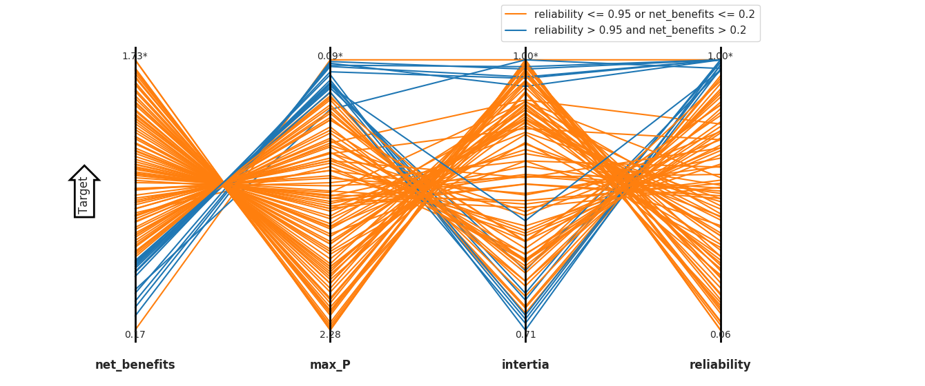
The variable paretoSet, is an instantiation of Rhodium’s DataSet class which now contains the Pareto approximate set found by NSGAII. We can visualize the approximate Pareto set using Rhodium’s built in visualization tools. Here I’ll use a Parallel Coordinate plot. Following Quinn et al., 2017, I’ll assume the stakeholders have set performance criteria of Reliability > 0.95 and Net Benefits > 0.2. Using Rhodium’s brushing functionality we can examine which solutions in our Pareto approximate set meet these criteria.

parallel_coordinates(model, paretoSet, target="top",
                           brush=[Brush("reliability > 0.95 and net_benefits > 0.2"), Brush("reliability <= 0.95 or net_benefits <= 0.2")])

Below, I’ve defined a function to evaluate a solution’s satisficing criteria. We can extract solutions that meet the criteria using the DataSet class’s find function.

criteria = lambda x : x["reliability"] > 0.95 and x["net_benefits"] > 0.2
acceptableSols = paretoSet.find(criteria)

DU Reevaluation

The solutions defined above meet stakeholder criteria if our assumptions about the state of the world (SOW) are correct, but what if the future deviates from our assumptions? To answer this question, I’ll create 1,000 new SOWs using latin hypercube sampling of our model uncertainties. I’ll then use Rhodium to reevaluate the set of acceptable solutions under each SOW (from here out I will refer to this as DU reevaluation). Rhodium has built in tools for both sampling uncertainties and reevaluating a set of solutions.

SOWs = sample_lhs(model, 1000)

reevaluation = [evaluate(model, update(SOWs, policy)) for policy in acceptableSols]

Measuring Robustness

For this exercise, I’ll examine four robustness measures reviewed in Herman et al., (2015). The four metrics include two variants of regret and two variants of satisficing, categories of robustness measures originally defined by Lempert and Collins, (2007). I’ll first show how each measure is calculated and how it can be coded in Rhodium, then I’ll illustrate how and why the choice of robustness metric changes the decision making process. All python implementations of robustness metrics in this post are adaptations of original functions written by Dave Hadka in the Rhodium source code.

Regret Type 1

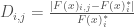
The first metric, regret type 1 (R1), measures a solution’s deviation from its performance in the baseline SOW. Examples of this metric’s use can be found in Kasprzyk et al., (2013) and Lempert and Collins, (2007). As defined by Herman et al., (2015), R1 measures robustness as the 90th percentile deviation in objective performance across SOWs, maximized across all objectives. The 90th percentile is used to capture tail performance while reducing susceptibility to outliers.

Where:

Where represents the value of objective i in the baseline SOW and represents the value of objective i calculated in SOW j.

Below I’ve coded a function which utilizes Rhodium’s built in data structures to calculate R1 for a given solution. The variable results is a Rhodium DataSet object containing the full set of DU reevaluations for one member of the Pareto approximate set. baseline is a DataSet containing the solution’s performance in the baseline state of the world.

def regret_type1(model, results, baseline, percentile=90):
    quantiles = []
    for response in model.responses:
        if response.dir == Response.MINIMIZE or response.dir == Response.MAXIMIZE:
            values = [abs((result[response.name] - baseline[response.name]) / baseline[response.name]) for result in results]
            quantiles.append(np.percentile(values, percentile))
            
    return max(quantiles)

Regret Type 2

Regret Type 2 (R2), is a variant of Savage regret introduced by Savage, 1951. R2 measures a decision maker’s regret for choosing a given solution over other available solutions by comparing the chosen solution’s performance in each SOW against the best performing option for that SOW. Like R1, R2 utilizes the 90th percentile deviation to capture tail behavior while reducing susceptibility to outliers:

Where:

if objective i is to be minimized and

if objective i is to be maximized.

The best value of each objective i is taken across the set of all solutions s. The deviation in R2 is normalized by the objective value itself rather than the best value, since this objective often approaches zero for minimization problems.

The function below again utilizes Rhodium’s data structures to efficiently implement a function for R2 in python. all_results is a list of DataSet objects, each containing the full set of DU reevaluations for one member of the Pareto approximate set. results is a DataSet containing the full set of DU reevaluations for the member of the Pareto approximate set being evaluated by this function.

def regret_type2(model, all_results, results, percentile=90):
    # for each uncertainty sampling, find the best value
    best = []
    
    for i in range(len(all_results[0])):
        entry = {}
        
        for response in model.responses:
            if response.dir == Response.MINIMIZE:
                entry[response.name] = min([result[response.name] for result in all_results])
            elif response.dir == Response.MAXIMIZE:
                entry[response.name] = max([result[response.name] for result in all_results])
                
        best.append(entry)
    
    # then compute the regret from the best value
    quantiles = []
    
    for response in model.responses:
        if response.dir == Response.MINIMIZE or response.dir == Response.MAXIMIZE:
            values = []
            
            for i in range(len(all_results[0])):
                values.append(abs((results[i][response.name] - best[i][response.name]) / results[i][response.name]))
            
            quantiles.append(np.percentile(values, percentile))
        
    return max(quantiles)

Satisficing Type 1

Satisficing metrics quantify a solution’s ability to meet prespecified performance criteria across deeply uncertain SOWs. Satisficing type 1, an approximation of Starr’s domain criterion (Starr 1962; Schneller and Sphicas, 1983) , represents the fraction of states of the world that a solution meets a set of performance criteria.

Where N is the number of sampled SOWs and = 1 if solution s meets the performance criteria in SOW j and = 0 otherwise. For this metric, we’ll utilize the performance criteria stated above: Relibility > 95% and Net Benefit > 0.2.

In python, we can express the performance criteria in a lambda function, as shown in the criteria function defined above. The function below calculates S1 for a solution whose DU reevaluation results have been stored in a DataSet objected called results.

def satisficing_type1(model, results, expr=None):
    # if no criteria are defined, check the feasibility across SOWs
    if expr is None:
        return mean(check_feasibility(model, results))
    # otherwise, return the number of SOWs that meet the specified criteria
    else:
        satisfactory = [expr(result) for result in results]
        return sum(satisfactory)/len(results)       

Satisficing Type 2

Satisficing type 2 (S2) is a measure of robustness derived from Info-Gap literature (Ben-Haim, 2004). S2 represents the uncertainty horizon that can be withstood before a solution fails to meet a set of performance criteria.

Where = maximum level of uncertainty, measured outward from the base SOW that can be tolerated before performance drops below threshold r*. In this example, I’ll normalize all uncertainties to their sampling range. In the function below, results is once again a Rhodium DataSet object containing the full set of DU reevaluations for one member of the Pareto approximate set. baseline is a DataSet containing the solution’s performance in the baseline state of the world. uncertainties_min is a list containing the lower bound for each uncertainty and uncertainties_max is a list containing upper bounds.

def satisficing_type2(model, results, baseline, uncertainties_max, uncertainties_min, expr=None):
    distances = []
    
    # ensure all default parameters are defined in baseline
    baseline = baseline.copy()
    populate_defaults(model, baseline)
    normalized_baseline = [baseline[u.name] for u in model.uncertainties]
    normalized_baseline = (np.array(uncertainties_max)-np.array(normalized_baseline))/(np.array(uncertainties_max)-np.array(uncertainties_min))
    
    for i, result in enumerate(results):
        if (expr is None and _is_feasible(model, result)) or (expr is not None and expr(result)==False):
            normalized_point = (np.array(uncertainties_max)- np.array([result[u.name] for u in model.uncertainties]))/(np.array(uncertainties_max)-np.array(uncertainties_min))
            distances.append(sp.distance.euclidean(
                    normalized_point,
                    normalized_baseline))
                      
    return 0.0 if len(distances) == 0 else min(distances)

Examining the results

• 

Figure 2: The top ranked solution according to each robustness measure along with each solution’s corresponding ranking across all other measures. Crossing lines indicate contrasting ordinal rankings of solution robustness between two measures. The preferablility of a solution is highly dependent on the choice of robustness metric.

Figure 2 shows the top ranked solution according to each robustness measure along with its corresponding rank across the other three measures. The four measures each provide different rankings of solution robustness. The top ranked solutions for the two regret based measures both preform poorly when evaluated under any of the other three measures, while the best solution according to S1 is tied for the best solution in S2 and ranks in the middle according to the two regret based solution. The second solution selected by S2 ranks at the bottom according to the other three metrics.

The disparity in ranking underscores the differences between the robustness measures. The wide difference in ranking between S2’s best solution and it’s ranking by the other three metrics indicates that while the uncertainties can deviate “far” from the base SOW before this solution fails, its performance is likely to be quite poor once this horizon is crossed. It’s poor ranking in S1 indicates that it will likely fail in many SOWs and it’s R1 ranking suggests that failures in the tail its performance are likely to be quite severe. Finally it’s low ranking in R2 means that there are other solutions that perform better across SOWs.

A solution that performs well by measure S2 may be preferable if decision makers have confidence that their assumptions about the base SOW are correct, however, this is rarely the case in conditions of deep uncertainty, so the solution recommended by S2 alone is likely undesirable. Furthermore, while S2 provides an aggregated measure of “distance to failure” this measure does not indicate which uncertainties drive failure or how far each individual uncertainty must deviate from the base SOW before the solution fails. A better way to understand a solution’s sensitivity to deeply uncertainties is through scenario discovery, which seeks to define vulnerable regions of the uncertainty space for a given solution. Rhodium has a set of built in scenario discovery tools, for details see this post by Julie.

The difference in robustness ranking between measures R1, R2 and S1 leave the decision makers with a choice regarding how they would like a solution to perform. Solutions that perform well in S1 maintain performance across the widest range of potential SOWs, but the metric provides no information on the severity of failure when the criteria is not met. Solutions that perform well in R1 are likely to have the least severe failures in the tails of their performance, but the metric does not measure the fraction of states of the world that result in poor performance. Measure R2 yields information about a solution’s performance relative to other options, but does not provide information about performance criteria or failure severity. As is often the case in decision making problems, the choice of measure should reflect a decision maker’s particular risk tolerance and preferences and must be tailored to each problem individually.

Final thoughts

This example has demonstrated how to use Rhodium to perform the first two steps of MORDM on a four objective formulation of the shallow lake problem. The results indicate that the choice of robustness metric changes which solutions are favored by decision makers. While I’ll wrap up this post here, this should not be the end of an MORDM analysis. After using the robustness metrics to select candidate policies, decision makers should perform scenario discovery to examine which uncertainties control solution performance and how these vulnerabilities differ between candidate solutions. Next, they should visualize each candidate policy to understand how it responds to various system states. Finally, they should think about whether these results necessitate any changes to the original problem formulation. If they choose to reformulate the problem, then the whole process starts back at the beginning. Luckily, Rhodium makes this process easy, allowing decision makers to examine problem formulations quickly and easily.

References

Ben-Haim, Y. (2004). “Uncertainty, probability and information-gaps.” Reliab. Eng. Syst. Saf., 85(1), 249–266.

Carpenter, S.R., Ludwig, D., Brock, W.A., 1999. Management of eutrophication for lakes subject to potentially irreversible change. Ecol. Appl. 9, 751e771.

Groves, D. G., and Lempert, R. J. (2007). “A new analytic method for finding policy-relevant scenarios.” Global Environ. Change, 17(1), 73–85.

Hall, J. W., Lempert, R. J., Keller, K., Hackbarth, A., Mijere, C., and
McInerney, D. J. (2012). “Robust climate policies under uncertainty:
A comparison of robust decision making and info-gap methods.”
Risk Anal., 32(10), 1657–1672

Herman, J.D., Reed, P.M., Zeff, H.B., Characklis, G.W., 2015. How should robustness be defined for water systems planning under change? J. Water Resour. Plan. Manag. 141, 04015012.

Kasprzyk, J. R., Nataraj, S., Reed, P. M., and Lempert, R. J. (2013). “Many objective robust decision making for complex environmental systems
undergoing change.” Environ. Modell. Softw., 42, 55–71.

Lempert, R. J., and Collins, M. (2007). “Managing the risk of an uncertain
threshold response: Comparison of robust, optimimum, and precaution-
ary approaches.” Risk Anal., 27(4), 1009–1026.

Matalas, N. C., and Fiering, M. B. (1977). “Water-resource systems
planning.” Climate, climatic change, and water supply, studies in geo-
physics, National Academy of Sciences, Washington, DC, 99–110.

Quinn, J. D., Reed, P. M., & Keller, K. (2017). Direct policy search for robust multi-objective management of deeply uncertain socio-ecological tipping points. Environmental Modelling & Software, 92, 125-141.

Savage, L. J. (1951). “The theory of statistical decision.” J. Am. Stat. Assoc., 46(253), 55–67.

Schneller, G., and Sphicas, G. (1983). “Decision making under uncertainty: Starr’s domain criterion.” Theory Decis., 15(4), 321–336.

Starr, M. K. (1962). Product design and decision theory, Prentice-Hall, Englewood Cliffs, NJ.

Spatial and temporal visualization of water demands in a basin

One of my main projects in the last couple years has been in the Upper Colorado River Basin, where we’ve been investigating how hundreds of water users in the basin might be affected by a variety of different changes and uncertainties that might take place in the region. Being in Colorado, water allocation in the basin follows prior-appropriation, where every user has a certain water right, defined by its seniority (where more senior = better) and its decree (i.e. how much water the right is granted for extraction). For the different users in the basin to receive water for their respective uses, prior-appropriation determines who gets X amount of water first based on seniority and given water availability, and then repeats down the seniority order until all requested water has been allocated. Hence, no user can extract water in a manner that affects any senior to them user.

During this investigation, we’ve been interested in seeing how this actually plays out through time and space in the basin, with the aim of potentially better understanding any consequential relationships that might exist between different users, as well as any emerging patterns that might be missed by looking at the data in a different manner. I tried to write a little script to do this in Python. I will be visualizing how users along the basin requested for some water at some historical month (the demand) and how much of that demand was actually met (the shortage), based on their right seniority and water availability in the basin.

There have been multiple posts in the blog on generating maps in Python (as well as in other languages), and they all use a module called Basemap which has been the most popular for these things, but it’s kinda buggy, and kinda a pain to install, and kinda a pain to get working, and I spent the better part of an entire workday to re-set it up on my machine and couldn’t. Enter Cartopy. After Basemap was announced deprecated, Cartopy was meant to be its replacement so I decided to transition. It was super easy to install and start generating maps within a couple minutes and the code I’ll be sharing today will be using that. I will also be using matplotlib’s animation classes to capture the water allocation to the different users through time in a video or a GIF.

First, I load up all necessary packages and data. structures contains the X and Y coordinates of all the diversion points; demands and shortages contain monthly data of water demand and shortage for each diversion point.

import numpy as np
import cartopy.feature as cpf
import cartopy.crs as ccrs
import matplotlib.pyplot as plt
import cartopy.io.img_tiles as cimgt
import pandas as pd
import matplotlib.animation as animation
import math

structures = pd.read_csv('modeled_diversions.csv',index_col=0)
demands = pd.read_csv('demands.csv',index_col=0)
shortages = pd.read_csv('shortages.csv',index_col=0)

Then, I set up the extent of my map (i.e., the region I would like to show). rivers_10m loads the river “feature” at a 10m resolution. There’s a lot of different features that can be added (coastlines, borders, etc.). Finally, I load the tiles which is basically the background map image (many other options also).

extent = [-109.069,-105.6,38.85,40.50]
rivers_10m = cpf.NaturalEarthFeature('physical', 'rivers_lake_centerlines', '10m')
tiles = cimgt.StamenTerrain()

I draw the figure more or less as I would in matplotlib, using the matplotlib scatter to draw my demand and shortage points. The rest of the lines are basically legend customization by creating dummy artists to show max demands and shortages in the legend.

fig = plt.figure(figsize=(12, 6))
ax = plt.axes(projection=tiles.crs)
ax.add_feature(rivers_10m, facecolor='None', edgecolor='b')
ax.add_image(tiles, 9, interpolation='none')
ax.set_extent(extent)
dem_points = ax.scatter(structures['X'], structures['Y'], marker = '.', s = demands['0']/50, c = 'dodgerblue', transform=ccrs.Geodetic())
short_points = ax.scatter(structures['X'], structures['Y'], marker = '.', s = shortages['0']/50, c = 'coral' ,transform=ccrs.Geodetic())
l2 = ax.scatter(-110,37, s=demands.values.max()/50, c = 'dodgerblue', transform=ccrs.Geodetic())
l4 = ax.scatter(-110,37, s=shortages.values.max()/50, c = 'coral',transform=ccrs.Geodetic())
dem_label = ax.scatter(-110,37, s=0, transform=ccrs.Geodetic())
short_label = ax.scatter(-110,37, s=0, transform=ccrs.Geodetic())
labels = ['Max Demand' , str(demands.values.max()) + ' af', 
          'Max Shortage' , str(shortages.values.max()) + ' af']
legend = ax.legend([dem_label, l2, short_label, l4], labels, ncol=2, loc = 'upper left', title = 'Month: '+ str((0 + 10) % 12 +1) + '/' + str(int(math.floor(0/12))+1908)+'\n', fontsize=10, title_fontsize = 14, borderpad=2, handletextpad = 1.3)

This code should produce something like the following, which shows the relative demand across users in blue, as well as how much of that demand was not met (shortage) in orange for November 1908. The large circles in the legend show the max demand and shortage across all users across all months in the record for reference.

To animate this, it’s very simple. All we need to create is another function (in this case update_points) that will define what changes at every frame of the animation. I’ve defined my function to adjust the size of every circle according to the timestep/frame, as well as change the title of the legend to the correct month. Matplotlib’s FuncAnimation then uses that and my figure to update it repeatedly (in this case for 120 steps). Finally, the animation can be saved to a video.

def update_points(num, dem_points, short_points, legend):
    dem_points.set_sizes(demands[str(num)]/10)
    short_points.set_sizes(shortages[str(num)]/10)
    legend.set_title('Month: '+ str((num + 10) % 12 +1) + '/' + str(int(math.floor(num/12))+1908))
    return dem_points, short_points, legend 
       
anim = animation.FuncAnimation(fig, update_points, 120, fargs=(dem_points, short_points, legend),
                                   interval=200, blit=False)
anim.save('basin_animation.mp4', fps=10,  dpi=150, extra_args=['-vcodec', 'libx264'])

WordPress reduces resolution, full res can be found here: https://imgur.com/a/6zfYIDU

There’s a lot to be added and improved, but from this simple version we can immediately see certain diversions popping out as well as geographical regions that exhibit frequent shortage. I will continue working on this and hopefully share improved versions in the future.

Parasol Resources

In my last post, I introduced Parasol: an open source, interactive parallel coordinates library for multi-objective decision making. For additional background on Parasol, check out the library’s webpage to view interactive example applications, the GitHub repo for documentation, and the paper [Raseman et al. (2019)] for a more rigorous overview of Parasol.

A demonstration of Parasol features like linked plots and data tables, highlighting individual polylines, and brushing and marking data.

In this post, I will describe how to start making your own interactive visualizations with Parasol.

Parasol Wiki

The best place to look for Parasol resources is the wiki page on the GitHub repo. Here you will find the API documentation, an introduction to web development for Parasol, and step-by-step tutorials taking you through the app development process. Because the wiki is likely to grow over time, I won’t provide links to these resources individually. Instead, I’ll give an overview of these resources here but I encourage you to visit the wiki for the most up-to-date tutorials and documentation.

API

The Application Programming Interface (API) is a list of all the features of the Parasol library. If you want to know everything that Parasol can do, the API is the perfect reference. If you are just getting started, however, this can be overwhelming. If that is the case, go through the tutorials and come back to the API page when you want to take your apps to the next level.

Web Development Basics

Creating Parasol apps requires some level of web development knowledge, but to build simple apps, you only need to understand the basics of HTML, JavaScript, and CSS. Check out the web development tutorial on the wiki for an overview of those concepts.

Tutorials

To start developing right away, go through the tutorials listed on the wiki page. These posts take the user through how to create a minimal Parasol app, they touch on the primary features of the API, and more advanced topics like how to use HTML buttons and sliders to create more polished apps.

Creating shareable apps with JSFiddle

Using JSFiddle to create shareable Parasol apps (without having to host them on a website)

I recently discovered JSFiddle–a sandbox tool for learning web development. Not only has JSFiddle made web development more accessible and easier for me to learn, but I realized its a great way to share Parasol apps in an efficient, informal way. Check out the tutorial on the wiki for more details and the following links to my own Parasol “fiddles”:

• Parasol Basic Example
• Parasol Tutorial #3 (Completed)

Give it a try!

As I’ve said before, check out Parasol and give us your feedback. If you think this library is valuable, submit an Issue or Star the GitHub repo, or write a comment below. We are open to new ideas and features about how Parasol can better suit the needs of developers.

References

Raseman, William J., Joshuah Jacobson, and Joseph R. Kasprzyk. “Parasol: An Open Source, Interactive Parallel Coordinates Library for Multi-Objective Decision Making.” Environmental Modelling & Software 116 (June 1, 2019): 153–63. https://doi.org/10.1016/j.envsoft.2019.03.005.