Ever installed a new library only for it to throw version depreciation errors up on your terminal? Or have warnings print in your output line instead of the figure you so painstakingly coded? Fear not – containerization is here to save the day! But before we get too excited, there are a few things (and terms) to learn about containerization using Docker.
In this post, we will be walking through a brief description of containerization and explain a few of its key terms. At the end, we will perform an exercise by containerizing the Rhodium robust decision-making library. More information about this library and how it can be used for exploratory modeling can be found in this post by Andrew Dircks. For a specific application of this library to the Lake Problem, please refer to this post by Antonia Hadjimichael.
Explaining containerization (and what is a base image?)
Using the image above, picture your hardware (laptop, desktop, supercomputer) as a large cargo ship, with its engines being its operating system. In the absence of containerization, an application (app) is developed in a specific computing environment, akin to placing cargo in a permanent storage hold under the deck of a ship. Methods for cargo loading and removal are strongly dictated by the shape and size of the ship. Similarly, a non-containerized app can only be reliably executed given that it is installed in a computing environment that is nearly or almost completely identical to that in which is was developed in.
On the contrary, containerization bundles everything an app might need to run in a ‘container’ – the code, its required libraries, and their associated dependencies – therefore enabling an app to be run consistently on any infrastructure. By extension, this renders a containerized application version- and operating system (OS)-independent. These ‘containers’ are thus easily loaded and installed onto any ‘cargo ship’. The piece of software that enables the efficient execution of containerized apps is the container engine. This nifty tool is responsible for handling app user input and ensuring the correct installation, startup and running of the containerized app. The engine also pulls, loads, and builds the container image, which is a (misleadingly-named) file, or repository of files, that contains all the information that the engine will need to build the app on a new machine.
In this post, we will be walking through the containerization of the Rhodium library using Docker, which is a container hub that let’s you develop, store and build your container images. It is the first and most commonly-used container hub (at the moment).
Let’s containerize!
Setup
If you use either a Windows or Mac machine, please install Docker Desktop from this site. Linux machines should first install Docker and then Docker Compose. Make sure to create an account and login.
Next, clone the PRIM, Platypus, and Rhodium repositories onto your local machine. You can directly download a .zip file of the repository here or you can clone the repository via your command line/terminal into a folder within a directory of your choice:
Great, your repositories are set and ready to go! These should result in three new folders: Rhodium, Platypus, and PRIM. Now, in the same terminal window, navigate to the PRIM folder and run the following:
Repeat for the Platypus folder. This is to make sure that you have both PRIM and Project Platypus installed and setup on your local machine.
Updating the requirements.txt file
Now, navigate back to the original directory-of-choice. Open the Rhodium folder, locate and open the requirements.txt file. Modify it so it looks like this:
matplotlib==3.5.1
numpy==1.22.1
pandas==1.4.0
mpldatacursor==0.7.1
six==1.16.0
scipy==1.7.3
prim
platypus-opt
sklearn==1.0.2
This file tells Docker that these are the required versions of libraries to install when building and installing your app.
Creating a Dockerfile
To begin building the container image for Docker to pack and build as Rhodium’s container, first create a new text file and name is Dockerfile within the Rhodium folder. Make sure to remove the .txt extension and save it as “All types” to avoid appending an extension. Open it using whichever text file you are comfortable with. The contents of this file should look like as follows. Note that the comments are for explanatory purposes only.
# state the base version of Python you are working with
# for my machine, it is Python 3.9.1
FROM python:3.9.1

# set the Rhodium repository as the container
WORKDIR /rhodium_app

# copy the requirements file into the new working directory
COPY requirements.txt .

# install all libraries and dependencies declared in the requirements file
RUN pip install -r requirements.txt

# copy the rhodium subfolder into the new working directory
# find this subfolder within the main Rhodium folder
COPY rhodium/ .

# this is the command the run when the container starts
CMD ["python", "./setup.py"]
The “.” indicates that you will be copying the file from your present directory into your working directory.
Build the Docker image
Once again in your terminal, check that you are in the same directory as before. Then, type in the following:
$ docker build -t rhodium_image .
Hit enter. If the containerization succeeded, you should see the following in your terminal (or something similar to it):
Containerization successful!
Congratulations, you have successfully containerized Rhodium! You are now ready for world domination!
Rhodium is a powerful, simple, open source Python library for multiobjective robust decision making. As part of Project Platypus, Rhodium is compatible with Platypus (a MOEA optimization library) and PRIM (the Patent Rule Induction Method for Python), making it a valuable tool for bridging optimization and analysis.
In the Rhodium documentation, a simple example of optimization and analysis uses the Lake Problem (DPS formulation). The actual optimization is performed in the line:
optimize(model, "NSGAII", 10000)
This optimize function uses the Platypus library directly for optimization; here the NSGAII algorithm is used for 10,000 function evaluations on the defined Lake Problem (model). This optimization call is concise and simple, but there are a few reasons why it may not be ideal.
Speed. Python, an interpreted language, is inherently slower than compiled languages (Java, C/C++, etc.) The Platypus library is built entirely in Python, making optimization slow.
Scalability. Platypus has support for parallelizing optimization, but this method is not ideal for large-scale computational experiments on computing clusters.
MOEA Suite. State of the art MOEAs such as the Borg MOEA are not implemented in Platypus for licensing reasons, so it is not usable directly by Rhodium.
Thus, external optimization is necessary for computationally demanding Borg runs. Luckily, Rhodium is easily compatible with external data files, so analysis with Rhodium of independent optimizations is simple. In this post, I’ll use a sample dataset obtained from a parallel Borg run of the Lake Problem, using the Borg wrapper.
The code and data used in this post can be found in this GitHub repository. lakeset.csv contains a Pareto approximate Lake Problem set. Each line is a solution, where the first six values are the decision variables and the last four are the corresponding objectives values.
We’ll use Pandas for data manipulation. The script below reads the sample .csv file with Pandas, converts it to a list of Python dictionaries, and creates a Rhodium DataSet. There are a few important elements to note. First, the Pandas to_dict function takes in an optional argument ‘records’to specify the format of the output. This specific format creates a list of Python dictionaries, where each element of the list is an individual solution (i.e. a line from the .csv file) with dictionary keys corresponding to the decision / objective value names and dictionary values as each line’s data. This is the format necessary for making a Rhodium DataSet, which we create by calling the constructor with the dictionary as input.
import pandas as pd
from rhodium import *

# use pandas to read the csv file
frame = pd.read_csv("lakeset.csv")

# convert the pandas data frame to a Python dict in record format
dictionary = frame.to_dict('records')

# create a Rhodium DataSet instance from the Python dictionary
dataset = DataSet(dictionary)
Printing the Rhodium DataSet with print(dataset)yields:
Once we have a Rhodium DataSet instantiated, we access many of the library’s functionalities, without performing direct optimization with Platypus. For example, if we want the policy with the lowest Phosphorus concentration (denoted by the ‘concentration’ field), the following code outputs:
Rhodium also offers powerful plotting functionalities. For example, we can easily create a Parallel Axis plot of our data to visualize the trade-offs between objectives. The following script uses the parallel_coordinates function in Rhodium on our external dataset. Here, since parallel_coordinatestakes a Rhodium model as input, we can: 1) define the external optimization problem as a Rhodium model, or 2) define a ‘dummy’ model that gives us just enough information to create plots. For the sake of simplicity, we will use the latter, but the first option is simple to set up if there exists a Python translation of your problem/model. Note, to access the scenario discovery and sensitivity analysis functionalities of Rhodium, it is necessary to create a real Rhodium Model.
# define a trivial "dummy" model in Rhodium with an arbitrary function
model = Model(lambda x: x)

# set up the model's objective responses to match the keys in your dataset
# here, all objectives are minimized
# this is the only information needed to create a parallel coordinate plot
model.responses = [Response("benefit", Response.MINIMIZE),
                   Response("concentration", Response.MINIMIZE),
                   Response("inertia", Response.MINIMIZE),
                   Response("reliability", Response.MINIMIZE)]

# create the parallel coordinate plot from the results of our external optimization
fig = parallel_coordinates(model, dataset, target="bottom",
                           brush=[Brush("reliability < -0.95"), Brush("reliability >= -0.95")])
TDLR; A Python implementation of grouped radial convergence plots based on code from the Rhodium library. This script is will be added to Antonia’s repository for Radial Convergence Plots.
Radial convergence plots are a useful tool for visualizing results of Sobol Sensitivities analyses. These plots array the model parameters in a circle and plot the first order, total order and second order Sobol sensitivity indices for each parameter. The first order sensitivity is shown as the size of a closed circle, the total order as the size of a larger open circle and the second order as the thickness of a line connecting two parameters.
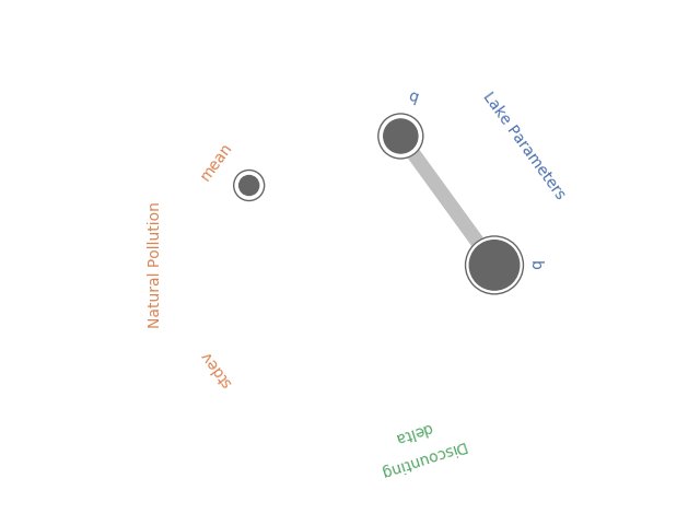
In May, Antonia created a new Python library to generate Radial Convergence plots in Python, her post can be found here and the Github repository here. I’ve been working with the Rhodium Library a lot recently and found that it contained a Radial Convergence Plotting function with the ability to plot grouped output, a functionality that is not present in Antonia’s repository. This function produces the same plots as Calvin’s R package. Adding a grouping functionality allows the user to color code the visualization to improve the interpretability of the results. In the code below I’ve adapted the Rhodium function to be a standalone Python code that can create visualizations from raw output of the SALib library. When used on a policy for the Lake Problem, the code generates the following plot shown in Figure 1.
Figure 1: Example Radial Convergence Plot for the Lake Problem reliability objective. Each of the points on the plot represents a sampled uncertain parameter in the model. The size of the filled circle represents the first order Sobol Sensitivity Index, the size of the open circle represents the total order Sobol Sensitivty Index and the thickness of lines between points represents the second order Sobol Sensitivity Index.
import numpy as np
import itertools
import matplotlib.pyplot as plt
import seaborn as sns
import math
sns.set_style('whitegrid', {'axes_linewidth': 0, 'axes.edgecolor': 'white'})

def is_significant(value, confidence_interval, threshold="conf"):
    if threshold == "conf":
        return value - abs(confidence_interval) > 0
    else:
        return value - abs(float(threshold)) > 0

def grouped_radial(SAresults, parameters, radSc=2.0, scaling=1, widthSc=0.5, STthick=1, varNameMult=1.3, colors=None, groups=None, gpNameMult=1.5, threshold="conf"):
    # Derived from https://github.com/calvinwhealton/SensitivityAnalysisPlots
    fig, ax = plt.subplots(1, 1)
    color_map = {}

    # initialize parameters and colors
    if groups is None:

        if colors is None:
            colors = ["k"]

        for i, parameter in enumerate(parameters):
            color_map[parameter] = colors[i % len(colors)]
    else:
        if colors is None:
            colors = sns.color_palette("deep", max(3, len(groups)))

        for i, key in enumerate(groups.keys()):
            #parameters.extend(groups[key])

            for parameter in groups[key]:
                color_map[parameter] = colors[i % len(colors)]

    n = len(parameters)
    angles = radSc*math.pi*np.arange(0, n)/n
    x = radSc*np.cos(angles)
    y = radSc*np.sin(angles)

    # plot second-order indices
    for i, j in itertools.combinations(range(n), 2):
        #key1 = parameters[i]
        #key2 = parameters[j]

        if is_significant(SAresults["S2"][i][j], SAresults["S2_conf"][i][j], threshold):
            angle = math.atan((y[j]-y[i])/(x[j]-x[i]))

            if y[j]-y[i] < 0:
                angle += math.pi

            line_hw = scaling*(max(0, SAresults["S2"][i][j])**widthSc)/2

            coords = np.empty((4, 2))
            coords[0, 0] = x[i] - line_hw*math.sin(angle)
            coords[1, 0] = x[i] + line_hw*math.sin(angle)
            coords[2, 0] = x[j] + line_hw*math.sin(angle)
            coords[3, 0] = x[j] - line_hw*math.sin(angle)
            coords[0, 1] = y[i] + line_hw*math.cos(angle)
            coords[1, 1] = y[i] - line_hw*math.cos(angle)
            coords[2, 1] = y[j] - line_hw*math.cos(angle)
            coords[3, 1] = y[j] + line_hw*math.cos(angle)

            ax.add_artist(plt.Polygon(coords, color="0.75"))

    # plot total order indices
    for i, key in enumerate(parameters):
        if is_significant(SAresults["ST"][i], SAresults["ST_conf"][i], threshold):
            ax.add_artist(plt.Circle((x[i], y[i]), scaling*(SAresults["ST"][i]**widthSc)/2, color='w'))
            ax.add_artist(plt.Circle((x[i], y[i]), scaling*(SAresults["ST"][i]**widthSc)/2, lw=STthick, color='0.4', fill=False))

    # plot first-order indices
    for i, key in enumerate(parameters):
        if is_significant(SAresults["S1"][i], SAresults["S1_conf"][i], threshold):
            ax.add_artist(plt.Circle((x[i], y[i]), scaling*(SAresults["S1"][i]**widthSc)/2, color='0.4'))

    # add labels
    for i, key in enumerate(parameters):
        ax.text(varNameMult*x[i], varNameMult*y[i], key, ha='center', va='center',
                rotation=angles[i]*360/(2*math.pi) - 90,
                color=color_map[key])

    if groups is not None:
        for i, group in enumerate(groups.keys()):
            print(group)
            group_angle = np.mean([angles[j] for j in range(n) if parameters[j] in groups[group]])

            ax.text(gpNameMult*radSc*math.cos(group_angle), gpNameMult*radSc*math.sin(group_angle), group, ha='center', va='center',
                rotation=group_angle*360/(2*math.pi) - 90,
                color=colors[i % len(colors)])

    ax.set_facecolor('white')
    ax.set_xticks([])
    ax.set_yticks([])
    plt.axis('equal')
    plt.axis([-2*radSc, 2*radSc, -2*radSc, 2*radSc])
    #plt.show()


    return fig
The code below implements this function using the SALib to conduct a Sobol Sensitivity Analysis on the Lake Problem to produce Figure 1.
import numpy as np
import itertools
import matplotlib.pyplot as plt
import math
from SALib.sample import saltelli
from SALib.analyze import sobol
from lake_problem import lake_problem
from grouped_radial import grouped_radial

# Define the problem for SALib
problem = {
	'num_vars': 5,
	'names': ['b', 'q', 'mean', 'stdev', 'delta'],
	'bounds': [[0.1, 0.45],
			   [2.0, 4.5],
			   [0.01, 0.05],
			   [0.001, 0.005],
			   [0.93, 0.99]]
}

# generate Sobol samples
param_samples = saltelli.sample(problem, 1000)

# extract each parameter for input into the lake problem
b_samples = param_samples[:,0]
q_samples = param_samples[:,1]
mean_samples = param_samples[:,2]
stdev_samples = param_samples[:,3]
delta_samples = param_samples[:,4]


# run samples through the lake problem using a constant policy of .02 emissions
pollution_limit = np.ones(100)*0.02

# initialize arrays to store responses
max_P = np.zeros(len(param_samples))
utility = np.zeros(len(param_samples))
inertia = np.zeros(len(param_samples))
reliability = np.zeros(len(param_samples))

# run model across Sobol samples
for i in range(0, len(param_samples)):
	print("Running sample " + str(i) + ' of ' + str(len(param_samples)))
	max_P[i], utility[i], inertia[i], reliability[i] = lake_problem(pollution_limit,
																	b=b_samples[i],
																	q=q_samples[i],
																	mean=mean_samples[i],
																	stdev=stdev_samples[i],
																	delta=delta_samples[i])

#Get sobol indicies for each response
SA_max_P = sobol.analyze(problem, max_P, print_to_console=False)
SA_reliability = sobol.analyze(problem, reliability, print_to_console=True)
SA_inertia = sobol.analyze(problem, inertia, print_to_console=False)
SA_utility = sobol.analyze(problem, utility, print_to_console=False)

# define groups for parameter uncertainties
groups={"Lake Parameters" : ["b", "q"],
        "Natural Pollution" : ["mean", "stdev"],
        "Discounting" : ["delta"]}


fig = grouped_radial(SA_reliability, ['b', 'q', 'mean', 'stdev', 'delta'], groups=groups, threshold=0.025)
plt.show()
Rhodium is a python library built to facilitate the Many Objective Robust Decision Making (MORM) framework. The MORDM framework couples many objective search with robust decision making (RDM) to facilitate decision support for complex, many-objective problems under deep uncertainty (Kasprzyk et al., 2013). A core component of MORDM is the quantification of robustness, which can be defined as “the insensitivity of system design to errors, random or otherwise, in the estimates of those parameters effecting design choice” (Matalas and Fiering, 1977; quote via Herman et al., 2015). While robustness as a concept may sound straightforward, quantifying robustness in mathematical terms is more challenging. As we’ll see later in this post, our choice on how to quantify robustness may have large implications on the decision making process. In this post I’ll demonstrate how to use Rhodium to examine the implications of the choice of robustness measure on the shallow lake problem from environmental systems literature. I’ll first walk through problem formulation and multi-objective optimization steps of MORDM, then implement four robustness metrics presented in Herman et al., (2015) on a set of candidate solutions.
Problem Formulation
The classical shallow lake problem (Carptenter et al,. 1999) presents a hypothetical town that seeks to balance economic benefits of phosphorus (P) emissions with the ecological benefits of a healthy lake. The lake naturally receives inflows of phosphorus from the surrounding area and recycles phosphorus in its system. Under natural conditions, the lake’s phosphorus levels will always return to a healthy (oligotrophic) equilibrium. However, if emissions from the town are too high, the lake will cross an irreversible tipping point into an unhealthy (eutrophic) state. The town seeks to find a policy to regulate phosphorus that will keep its economy prosperous while preserving a healthy ecosystem.
System Model
To facilitate the decision making process, decision makers employ a dimensionless model to abstract phosphorus dynamics in the lake:
Where X is the normalized concentration of P in the lake, a represents the anthropogenic phosphorus inputs from the town, Y ~ LN(mu, sigma) are natural P inputs to the lake, q is a parameter controlling the recycling rate of P from sediment, b is a parameter controlling the rate at which P is removed from the system and t is the time index in years. For details on the lake problem model, see Quinn et al., (2017).
Uncertainties
Decision makers have estimates of model parameters that govern the flux of phosphorus, however, these parameters are uncertain and their probability distributions are unknown, therefore they are treated as deep uncertainties. The assumed values and plausible ranges of these uncertainties are shown in the table below.
Uncertainty
Base Value
Lower bound
Upper Bound
b
0.42
0.1
0.45
q
2.0
2.0
4.5
delta
0.98
0.93
0.99
mu
0.03
0.01
0.05
sigma
(10^-5)^.5
0.001
0.005
Objectives
Local stakeholders have identified four objectives they would like to optimize:
Maximize the average economic benefit of phosphorus emissions
Minimize the worst case average phosphorus concentration in the lake
Maximize the inertia of the phosphorus control policy (ie. do not create a policy with large year to year swings in phosphorus emissions)
Maximize the reliability of a policy staying below the lake’s critical phosphorus threshold
For details on the objective formulations, refer to Quinn et al., (2017).
Decisions
Following Quinn et al., (2017), phosphorus emissions are controlled by a state dependent rule system which uses cubic radial basis functions to determine annual phosphorus emissions based on the phosphorus in the lake.
Where , and are the centers, radii and wights of n cubic radial basis functions. These parameters will be the decision variables for our multi-objective optimization (searching for parameters to a rule system like this is known as direct policy search (DPS)). For this example we’ll use n=2 cubic radial basis functions and have 6 decision variables.
Building the model in Rhodium
Conducting MORDM on your own can be an onerous process, often your model is written in a different language than you post-processing software and each individual script requires data in a different format. Rhodium can make the MORDM process much easier. It has custom built data structures which are tailored for MORDM analysis and a declarative structure which makes plugging in an external model simple. For this demonstration I’ll use a python implementation of the Lake problem which I’ve copied to this Git repository (to save space I’m omitting it from the text of this post). The first step in conducting MORDM with Rhodium is to declare a Rhodium model. This file must be in the same repository as the python file running rhodium, I’ll also need the file RBFpolicy.py, found here.
model = Model(LakeProblemDPS)
To properly declare the model I need to specify model parameters, levers, uncertainties and model responses. Model parameters include any input that will change across model evaluations. I also need to let Rhodium know which parameters are decision variables or “levers” and which are uncertainties. I can do this by explicitly declaring levers, uncertainties and their ranges as shown below.
Next, I need to specify model responses. Model responses include any optimization objective and any information needed to assess constraints or other information. When specifying output I also need to tell Rhodium what kind of response each variable represents (ie minimize or maximize etc.).
Now that I’ve defined our model, I’m ready to perform search with an MOEA. In this example I’ll use NSGAII and search over 10,000 function evaluations. This optimization takes a long time when running in serial, so I’ll exploit Rhodium’s parallelization capabilities to utilize 4 core on my desktop computer.
# Use a Process Pool evaluator, which will work on Python 3+
if __name__ == "__main__":
    with ProcessPoolEvaluator(4) as evaluator:
        RhodiumConfig.default_evaluator = evaluator
        paretoSet = optimize(model, "NSGAII", 10000)
The variable paretoSet, is an instantiation of Rhodium’s DataSet class which now contains the Pareto approximate set found by NSGAII. We can visualize the approximate Pareto set using Rhodium’s built in visualization tools. Here I’ll use a Parallel Coordinate plot. Following Quinn et al., 2017, I’ll assume the stakeholders have set performance criteria of Reliability > 0.95 and Net Benefits > 0.2. Using Rhodium’s brushing functionality we can examine which solutions in our Pareto approximate set meet these criteria.
parallel_coordinates(model, paretoSet, target="top",
                           brush=[Brush("reliability > 0.95 and net_benefits > 0.2"), Brush("reliability <= 0.95 or net_benefits <= 0.2")])
Below, I’ve defined a function to evaluate a solution’s satisficing criteria. We can extract solutions that meet the criteria using the DataSet class’s find function.
criteria = lambda x : x["reliability"] > 0.95 and x["net_benefits"] > 0.2
acceptableSols = paretoSet.find(criteria)
DU Reevaluation
The solutions defined above meet stakeholder criteria if our assumptions about the state of the world (SOW) are correct, but what if the future deviates from our assumptions? To answer this question, I’ll create 1,000 new SOWs using latin hypercube sampling of our model uncertainties. I’ll then use Rhodium to reevaluate the set of acceptable solutions under each SOW (from here out I will refer to this as DU reevaluation). Rhodium has built in tools for both sampling uncertainties and reevaluating a set of solutions.
SOWs = sample_lhs(model, 1000)

reevaluation = [evaluate(model, update(SOWs, policy)) for policy in acceptableSols]
Measuring Robustness
For this exercise, I’ll examine four robustness measures reviewed in Herman et al., (2015). The four metrics include two variants of regret and two variants of satisficing, categories of robustness measures originally defined by Lempert and Collins, (2007). I’ll first show how each measure is calculated and how it can be coded in Rhodium, then I’ll illustrate how and why the choice of robustness metric changes the decision making process. All python implementations of robustness metrics in this post are adaptations of original functions written by Dave Hadka in the Rhodium source code.
Regret Type 1
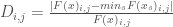
The first metric, regret type 1 (R1), measures a solution’s deviation from its performance in the baseline SOW. Examples of this metric’s use can be found in Kasprzyk et al., (2013) and Lempert and Collins, (2007). As defined by Herman et al., (2015), R1 measures robustness as the 90th percentile deviation in objective performance across SOWs, maximized across all objectives. The 90th percentile is used to capture tail performance while reducing susceptibility to outliers.
Where:
Where represents the value of objective i in the baseline SOW and represents the value of objective i calculated in SOW j.
Below I’ve coded a function which utilizes Rhodium’s built in data structures to calculate R1 for a given solution. The variable results is a Rhodium DataSet object containing the full set of DU reevaluations for one member of the Pareto approximate set. baseline is a DataSet containing the solution’s performance in the baseline state of the world.
def regret_type1(model, results, baseline, percentile=90):
    quantiles = []
    for response in model.responses:
        if response.dir == Response.MINIMIZE or response.dir == Response.MAXIMIZE:
            values = [abs((result[response.name] - baseline[response.name]) / baseline[response.name]) for result in results]
            quantiles.append(np.percentile(values, percentile))

    return max(quantiles)
Regret Type 2
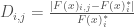
Regret Type 2 (R2), is a variant of Savage regret introduced by Savage, 1951. R2 measures a decision maker’s regret for choosing a given solution over other available solutions by comparing the chosen solution’s performance in each SOW against the best performing option for that SOW. Like R1, R2 utilizes the 90th percentile deviation to capture tail behavior while reducing susceptibility to outliers:
Where:
if objective i is to be minimized and
if objective i is to be maximized.
The best value of each objective i is taken across the set of all solutions s. The deviation in R2 is normalized by the objective value itself rather than the best value, since this objective often approaches zero for minimization problems.
The function below again utilizes Rhodium’s data structures to efficiently implement a function for R2 in python. all_results is a list of DataSet objects, each containing the full set of DU reevaluations for one member of the Pareto approximate set. results is a DataSet containing the full set of DU reevaluations for the member of the Pareto approximate set being evaluated by this function.
def regret_type2(model, all_results, results, percentile=90):
    # for each uncertainty sampling, find the best value
    best = []

    for i in range(len(all_results[0])):
        entry = {}

        for response in model.responses:
            if response.dir == Response.MINIMIZE:
                entry[response.name] = min([result[response.name] for result in all_results])
            elif response.dir == Response.MAXIMIZE:
                entry[response.name] = max([result[response.name] for result in all_results])

        best.append(entry)

    # then compute the regret from the best value
    quantiles = []

    for response in model.responses:
        if response.dir == Response.MINIMIZE or response.dir == Response.MAXIMIZE:
            values = []

            for i in range(len(all_results[0])):
                values.append(abs((results[i][response.name] - best[i][response.name]) / results[i][response.name]))

            quantiles.append(np.percentile(values, percentile))

    return max(quantiles)
Satisficing Type 1
Satisficing metrics quantify a solution’s ability to meet prespecified performance criteria across deeply uncertain SOWs. Satisficing type 1, an approximation of Starr’s domain criterion (Starr 1962; Schneller and Sphicas, 1983) , represents the fraction of states of the world that a solution meets a set of performance criteria.
Where N is the number of sampled SOWs and = 1 if solution s meets the performance criteria in SOW j and = 0 otherwise. For this metric, we’ll utilize the performance criteria stated above: Relibility > 95% and Net Benefit > 0.2.
In python, we can express the performance criteria in a lambda function, as shown in the criteria function defined above. The function below calculates S1 for a solution whose DU reevaluation results have been stored in a DataSet objected called results.
def satisficing_type1(model, results, expr=None):
    # if no criteria are defined, check the feasibility across SOWs
    if expr is None:
        return mean(check_feasibility(model, results))
    # otherwise, return the number of SOWs that meet the specified criteria
    else:
        satisfactory = [expr(result) for result in results]
        return sum(satisfactory)/len(results)
Satisficing Type 2
Satisficing type 2 (S2) is a measure of robustness derived from Info-Gap literature (Ben-Haim, 2004). S2 represents the uncertainty horizon that can be withstood before a solution fails to meet a set of performance criteria.
Where = maximum level of uncertainty, measured outward from the base SOW that can be tolerated before performance drops below threshold r*. In this example, I’ll normalize all uncertainties to their sampling range. In the function below, results is once again a Rhodium DataSet object containing the full set of DU reevaluations for one member of the Pareto approximate set. baseline is a DataSet containing the solution’s performance in the baseline state of the world. uncertainties_min is a list containing the lower bound for each uncertainty and uncertainties_max is a list containing upper bounds.
def satisficing_type2(model, results, baseline, uncertainties_max, uncertainties_min, expr=None):
    distances = []

    # ensure all default parameters are defined in baseline
    baseline = baseline.copy()
    populate_defaults(model, baseline)
    normalized_baseline = [baseline[u.name] for u in model.uncertainties]
    normalized_baseline = (np.array(uncertainties_max)-np.array(normalized_baseline))/(np.array(uncertainties_max)-np.array(uncertainties_min))

    for i, result in enumerate(results):
        if (expr is None and _is_feasible(model, result)) or (expr is not None and expr(result)==False):
            normalized_point = (np.array(uncertainties_max)- np.array([result[u.name] for u in model.uncertainties]))/(np.array(uncertainties_max)-np.array(uncertainties_min))
            distances.append(sp.distance.euclidean(
                    normalized_point,
                    normalized_baseline))

    return 0.0 if len(distances) == 0 else min(distances)
Examining the results
Figure 2: The top ranked solution according to each robustness measure along with each solution’s corresponding ranking across all other measures. Crossing lines indicate contrasting ordinal rankings of solution robustness between two measures. The preferablility of a solution is highly dependent on the choice of robustness metric.
Figure 2 shows the top ranked solution according to each robustness measure along with its corresponding rank across the other three measures. The four measures each provide different rankings of solution robustness. The top ranked solutions for the two regret based measures both preform poorly when evaluated under any of the other three measures, while the best solution according to S1 is tied for the best solution in S2 and ranks in the middle according to the two regret based solution. The second solution selected by S2 ranks at the bottom according to the other three metrics.
The disparity in ranking underscores the differences between the robustness measures. The wide difference in ranking between S2’s best solution and it’s ranking by the other three metrics indicates that while the uncertainties can deviate “far” from the base SOW before this solution fails, its performance is likely to be quite poor once this horizon is crossed. It’s poor ranking in S1 indicates that it will likely fail in many SOWs and it’s R1 ranking suggests that failures in the tail its performance are likely to be quite severe. Finally it’s low ranking in R2 means that there are other solutions that perform better across SOWs.
A solution that performs well by measure S2 may be preferable if decision makers have confidence that their assumptions about the base SOW are correct, however, this is rarely the case in conditions of deep uncertainty, so the solution recommended by S2 alone is likely undesirable. Furthermore, while S2 provides an aggregated measure of “distance to failure” this measure does not indicate which uncertainties drive failure or how far each individual uncertainty must deviate from the base SOW before the solution fails. A better way to understand a solution’s sensitivity to deeply uncertainties is through scenario discovery, which seeks to define vulnerable regions of the uncertainty space for a given solution. Rhodium has a set of built in scenario discovery tools, for details see this post by Julie.
The difference in robustness ranking between measures R1, R2 and S1 leave the decision makers with a choice regarding how they would like a solution to perform. Solutions that perform well in S1 maintain performance across the widest range of potential SOWs, but the metric provides no information on the severity of failure when the criteria is not met. Solutions that perform well in R1 are likely to have the least severe failures in the tails of their performance, but the metric does not measure the fraction of states of the world that result in poor performance. Measure R2 yields information about a solution’s performance relative to other options, but does not provide information about performance criteria or failure severity. As is often the case in decision making problems, the choice of measure should reflect a decision maker’s particular risk tolerance and preferences and must be tailored to each problem individually.
Final thoughts
This example has demonstrated how to use Rhodium to perform the first two steps of MORDM on a four objective formulation of the shallow lake problem. The results indicate that the choice of robustness metric changes which solutions are favored by decision makers. While I’ll wrap up this post here, this should not be the end of an MORDM analysis. After using the robustness metrics to select candidate policies, decision makers should perform scenario discovery to examine which uncertainties control solution performance and how these vulnerabilities differ between candidate solutions. Next, they should visualize each candidate policy to understand how it responds to various system states. Finally, they should think about whether these results necessitate any changes to the original problem formulation. If they choose to reformulate the problem, then the whole process starts back at the beginning. Luckily, Rhodium makes this process easy, allowing decision makers to examine problem formulations quickly and easily.
References
Ben-Haim, Y. (2004). “Uncertainty, probability and information-gaps.” Reliab. Eng. Syst. Saf., 85(1), 249–266.
Carpenter, S.R., Ludwig, D., Brock, W.A., 1999. Management of eutrophication for lakes subject to potentially irreversible change. Ecol. Appl. 9, 751e771.
Groves, D. G., and Lempert, R. J. (2007). “A new analytic method for finding policy-relevant scenarios.” Global Environ. Change, 17(1), 73–85.
Hall, J. W., Lempert, R. J., Keller, K., Hackbarth, A., Mijere, C., and McInerney, D. J. (2012). “Robust climate policies under uncertainty: A comparison of robust decision making and info-gap methods.” Risk Anal., 32(10), 1657–1672
Herman, J.D., Reed, P.M., Zeff, H.B., Characklis, G.W., 2015. How should robustness be defined for water systems planning under change? J. Water Resour. Plan. Manag. 141, 04015012.
Kasprzyk, J. R., Nataraj, S., Reed, P. M., and Lempert, R. J. (2013). “Many objective robust decision making for complex environmental systems undergoing change.” Environ. Modell. Softw., 42, 55–71.
Lempert, R. J., and Collins, M. (2007). “Managing the risk of an uncertain threshold response: Comparison of robust, optimimum, and precaution- ary approaches.” Risk Anal., 27(4), 1009–1026.
Matalas, N. C., and Fiering, M. B. (1977). “Water-resource systems
planning.” Climate, climatic change, and water supply, studies in geo-
physics, National Academy of Sciences, Washington, DC, 99–110.
Quinn, J. D., Reed, P. M., & Keller, K. (2017). Direct policy search for robust multi-objective management of deeply uncertain socio-ecological tipping points. Environmental Modelling & Software, 92, 125-141.
Savage, L. J. (1951). “The theory of statistical decision.” J. Am. Stat. Assoc., 46(253), 55–67.
Schneller, G., and Sphicas, G. (1983). “Decision making under uncertainty: Starr’s domain criterion.” Theory Decis., 15(4), 321–336.
Starr, M. K. (1962). Product design and decision theory, Prentice-Hall, Englewood Cliffs, NJ.
TLDR; Python script for radial convergence plots that can be found here.
You might have encountered this type of graph before, they’re usually used to present relationships between different entities/parameters/factors and they typically look like this:
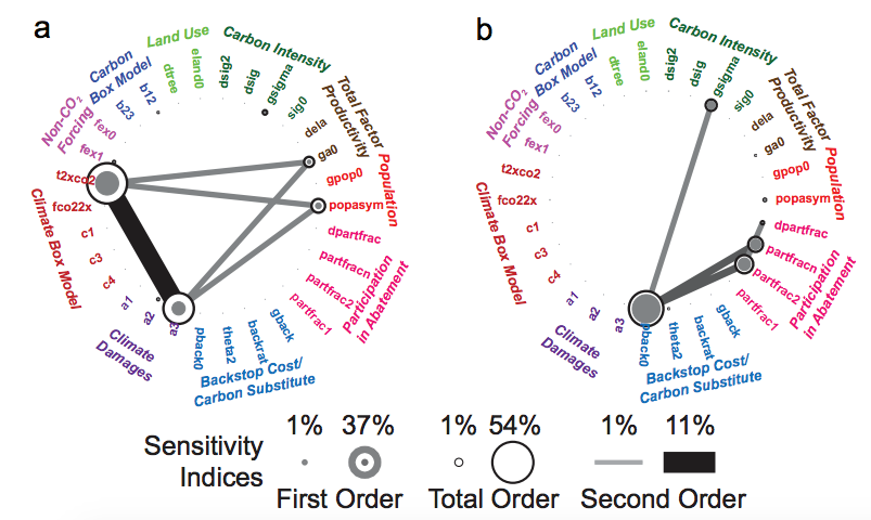
In the context of our work, I have seen them used to present sensitivity analysis results, where we are interested in both the individual significance of a model parameter, but also the extent of its interaction with others. For example, in Butler et al. (2014) they were used to present First, Second, and Total order parameter sensitivities as produced by a Sobol’ Sensitivity Analysis.
From Butler et al. (2014)
I set out to write a Python script to replicate them. Calvin Whealton has written a similar script in R, and the same functionality also exists within Rhodium. I just wanted something with a bit more flexibility, so I wrote this script that produces two types of these graphs, one with straight lines and one with curved (which are prettier IMO). The script takes dictionary items as inputs, either directly from SALib and Rhodium (if you are using it to display Sobol results), or by importing them (to display anything else). You’ll need one package to get this to run: NetworkX. It facilitates the organization of the nodes in a circle and it’s generally a very stable and useful package to have.
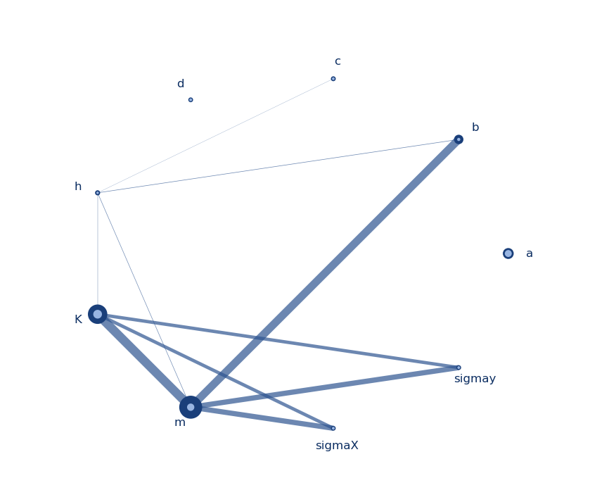
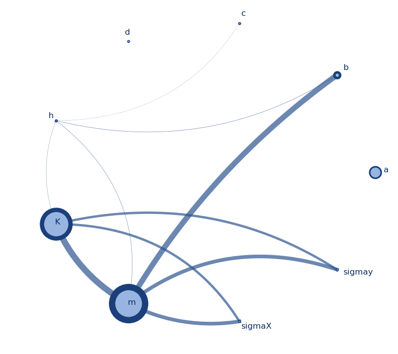
Graph with straight linesGraph with curved lines
I made these graphs to display results the results of a Sobol analysis I performed on the model parameters of a system I am studying (a, b, c, d, h, K, m, sigmax, and sigmay). The node size indicates the first order index (S1) per parameter, the node border thickness indicates the total order index (ST) per parameter, and the thickness of the line between two nodes indicates the secord order index (S2). The colors, thicknesses, and sizes can be easily changed to fit your needs. The script for these can be found here, and I will briefly discuss what it does below.
After loading the necessary packages (networkx, numpy, itertools, and matplotlib) and data, there is some setting parameters that can be adapted for the figure generation. First, we can define a significance value for the indices (here set to 0.01). To keep all values just set it to 0. Then we have some stylistic variables that basically define the thicknesses and sizes for the lines and nodes. They can be changed to get the look of the graph to your liking.
# Set min index value, for the effects to be considered significant
index_significance_value = 0.01
node_size_min = 15 # Max and min node size
node_size_max = 30
border_size_min = 1 # Max and min node border thickness
border_size_max = 8
edge_width_min = 1 # Max and min edge thickness
edge_width_max = 10
edge_distance_min = 0.1 # Max and min distance of the edge from the center of the circle
edge_distance_max = 0.6 # Only applicable to the curved edges
The rest of the code should just do the work for you. It basically does the following:
Define basic variables and functions that help draw circles and curves, get angles and distances between points
Set up graph with all parameters as nodes and draw all second order (S2) indices as lines (edges in the network) connecting the nodes. For every S2 index, we need a Source parameter, a Target parameter, and the Weight of the line, given by the S2 index itself. If you’re using this script for other data, different information can fit into the line thickness, or they could all be the same.
Draw nodes and lines in a circular shape and adjust node sizes, borders, and line thicknesses to show the relative importance/weight. Also, annotate text labels on each node and adjust their location accordingly. This produces the graph with the straight lines.
For the graph with the curved lines, define function that will generate the x and y coordinates for them, and then plot using matplotlib.
I would like to mention this script by Enrico Ubaldi, based on which I developed mine.


 ,
,  and
and  are the centers, radii and wights of n cubic radial basis functions. These parameters will be the decision variables for our multi-objective optimization (searching for parameters to a rule system like this is known as direct policy search (DPS)). For this example we’ll use n=2 cubic radial basis functions and have 6 decision variables.
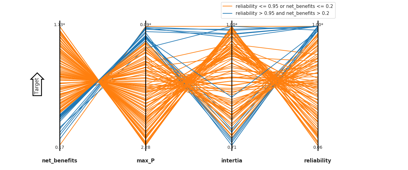
![R1 = \max_i[D_{i,90}:P(D_i\leq D_{i,90}=0.90]](https://s0.wp.com/latex.php?latex=R1+%3D+%5Cmax_i%5BD_%7Bi%2C90%7D%3AP%28D_i%5Cleq+D_%7Bi%2C90%7D%3D0.90%5D&bg=ffffff&fg=444444&s=0&c=20201002)
 represents the value of objective i in the baseline SOW and
  represents the value of objective i calculated in SOW j.
 ![R2 = \max_i[D_{i,90}:P(D_i\leq D_{i,90}=0.90]](https://s0.wp.com/latex.php?latex=R2+%3D+%5Cmax_i%5BD_%7Bi%2C90%7D%3AP%28D_i%5Cleq+D_%7Bi%2C90%7D%3D0.90%5D&bg=ffffff&fg=444444&s=0&c=20201002)


 = 1 if solution s meets the performance criteria in SOW j and
 ![S2 = \hat{\alpha} = max \big[\alpha:min_{j \in U(\alpha)} F(x)_j \geq r^* \big]](https://s0.wp.com/latex.php?latex=S2+%3D+%5Chat%7B%5Calpha%7D+%3D+max+%5Cbig%5B%5Calpha%3Amin_%7Bj+%5Cin+U%28%5Calpha%29%7D+F%28x%29_j+%5Cgeq+r%5E%2A+%5Cbig%5D&bg=ffffff&fg=444444&s=0&c=20201002)
 = maximum level of uncertainty, measured outward from the base SOW that can be tolerated before performance drops below threshold r*. In this example, I’ll normalize all uncertainties to their sampling range. In the function below, results is once again a Rhodium DataSet object containing the full set of DU reevaluations for one member of the Pareto approximate set. baseline is a DataSet containing the solution’s performance in the baseline state of the world. uncertainties_min is a list containing the lower bound for each uncertainty and uncertainties_max is a list containing upper bounds.