In this blog post, we will be reviewing how to perform runtime diagnostics using MOEAFramework. This software has been used in prior blog posts by Rohini and Jazmin to perform MOEA diagnostics across multiple MOEA parameterizations. Since then, MOEAFramework has undergone a number of updates and structure changes. This blog post will walk through the updated functionality of running MOEAFramework (version 4.0) via the command line to perform runtime diagnostics across 20 seeds using one set of parameters. We will be using the classic 3-objective DTLZ2 problem optimized using NSGAII, both of which are in-built into MOEAFramework.
Before we begin, some helpful tips and system configuration requirements:
Ensure that you have the latest version of Java installed (as of April 2024, this is Java Version 22). The current version of MOEAFramework was compiled using class file version 61.0, which was made available in Java Version 17 (find the complete list of Java versions and their associated class files here). This is the minimum requirement for being able to run MOEAFramework.
The following commands are written for a Linux interface. Download a Unix terminal emulator like Cygwin if needed.
Another helpful tip: to see all available flags and their corresponding variables, you can use the following structure:
For the a full list of parameter files for each of the in-built MOEAFramework algorithms, please see Jazmin’s post here.
In this example, I have called it NSGAII_Params.txt. Note that maxEvaluations is set to 10,000 on both its lower and upper bounds. This is because we want to fix the number of function evaluations completed by NSGAII. Next, in our command line, we run:
The output NSGAII_Latin file should contain a single-line that can be opened as a text file. It should have six tab-delineated values that correspond to the six parameters in the input file that you have generated. Now that you have your MOEA parameter files, let’s begin running some optimizations!
First, make a new folder in your current directory to store your output data. Here, I am simply calling it data.
mkdir data
Next, optimize the DTLZ2 3-objective problem using NSGAII:
for i in {1..20}; do java -cp MOEAFramework-4.0-Demo.jar org.moeaframework.analysis.tools.RuntimeEvaluator --parameterFile NSGAII_Params.txt --input NSGAII_Latin --problem DTLZ2_3 --seed $i --frequency 1000 --algorithm NSGAII --output data/NSGAII_DTLZ2_3_$i.data; done
Here’s what’s going down:
First, you are performing a runtime evaluation of the optimization of the 3-objective DTLZ2 problem using NSGAII
You are obtaining the decision variables and objective values at every 1,000 function evaluations, effectively tracking the progress of NSGAII as it attempts to solve the problem
Finally, you are storing the output in the data/ folder
You then repeat this for 20 seeds (or for as many as you so desire).
Double check your .data file. It should contain information on your decision variables and objective values at every 1,000 NFEs or so, seperated from the next thousand by a “#”.
Generate the reference set
Next, obtain the only the objective values at every 1,000 NFEs by entering the following into your command line:
for i in {1..20}; do java -cp MOEAFramework-4.0-Demo.jar org.moeaframework.analysis.tools.ResultFileMerger --problem DTLZ2_3 --output data/NSGAII_DTLZ2_3_$i.set --epsilon 0.01,0.01,0.01 data/NSGAII_DTLZ2_3_$i.data; done
Notice that we have a new flag here – the --epsilon flag tells MOEAFramework that you only want objective values that are at least 0.01 better than other non-dominated objective values for a given objective. This helps to trim down the size of the final reference set (coming up soon) and remove solutions that are only marginally better (and may not be decision-relevant in the real-world context).
On to generating the reference set – let’s combine all objectives across all seeds using the following command line directive:
for i in {1..20}; do java -cp MOEAFramework-4.0-Demo.jar org.moeaframework.analysis.tools.ReferenceSetMerger --output data/NSGAII_DTLZ2_3.ref -epsilon 0.01,0.01,0.01 data/NSGAII_DTLZ2_3_$i.set; done
Your final reference set should now be contained within the NSGAII_DTLZ2_3.ref file in the data/ folder.
Generate the runtime metrics
Finally, let’s generate the runtime metrics. To avoid any mix-ups, let’s create a folder to store these files:
mkdir data_metrics
And finally, generate our metrics!
or i in {1..20}; do java -cp MOEAFramework-4.0-Demo.jar org.moeaframework.analysis.tools.ResultFileEvaluator --problem DTLZ2_3 --epsilon 0.01,0.01,0.01 --input data/NSGAII_DTLZ2_3_$i.data --reference data/NSGAII_DTLZ2_3.ref --output data_metrics/NSGAII_DTLZ2_3_$i.metrics; done
If all goes well, you should see 20 files (one each for each seed) similar in structure to the one below in your data_metrics/ folder:
The header values are the names of each of the MOEA performance metrics that MOEAFramework measures. In this blog post, we will proceed with visualizing the hypervolume over time across all 20 seeds.
Visualizing runtime diagnostics
The following Python code first extracts the metric that you would like to view, and saves the plot as a PNG file in the data_metrics/ folder:
If you correctly implemented the code, you should be able to be view the following figure that shows how the hypervolume attained by the NSGAII algorithm improves steadily over time.
In the figure above, the colored inner region spans the hypervolume attained across all 20 seeds, with the dotted line representing the mean hypervolume over time. The solid upper and lower bounding lines are the maximum and minimum hypervolume achieved every 1,000 NFEs respectively. Note that, in this specific instance, NSGAII only achieves about 50% of the total hypervolume of the overall objective space. This implies that a higher NFE (a longer runtime) is required for NSGAII to further increase the hypervolume achieved. Nonetheless, the rate of hypervolume increase is gradually decreasing, indicating that this particular parameterization of NSGAII is fast approaching its maximum possible hypervolume, which additional NFEs only contributing small improvements to performance. It is also worth noting the narrow range of hypervolume values, especially as the number of NFEs grows larger. This is representative of the reliability of the NGSAII algorithm, demonstrating that is can somewhat reliably reproduce results across multiple different seeds.
Summary
This just about brings us to the end of this blog post! We’ve covered how to perform MOEA runtime diagnostics and plot the results. If you are curious, here are some additional things to explore:
Plot different performance metrics against NFE. Please see Joe Kasprzyk’s post here to better understand the plots you generate.
Explore different MOEAs that are built into MOEAFramework to see how they perform across multiple seeds.
Generate multiple MOEA parameter samples using the in-built MOEAFramework Latin Hypercube Sampler to analyze the sensitivity of a given MOEA to its parameterization.
Attempt examining the runtime diagnostics of Borg MOEA using the updated version of MOEAFramework.
On that note, make sure to check back for updates as MOEAFramework is being actively reviewed and improved! You can view the documentation of Version 4.0 here and access its GitHub repository here.
In this blog post, we will be discussing the many household uses of citrus aurantiifolio, or the common lime.
Just kidding, we’ll be talking about a completely different type of LIME, namely Local Interpretable Model-Agnostic Explanations (at this point you may be thinking that the former’s scientific name becomes the easier of the two to say). After all, this is the WaterProgramming blog.
On a more serious note though, LIME is one of the two widely-known model agnostic explainable AI (xAI) methods, alongside Shapley Additive Explanations (SHAP). This post is intended to be an introduction to LIME in particular, and we will be setting up the motivation for using xAI methods as well as a brief example application using the North Carolina Research Triangle system.
Before we proceed, here’s a quick graphic to get oriented:
The figure above mainly demonstrates three main concepts: Artificial Intelligence (AI), the methods used to achieve AI (one of which includes Machine Learning, or ML), and the methods to explain how such methods achieved their version of AI (explainable AI, or more catchily known as xAI). For more explanation on the different categories of AI, and their methods, please refer to these posts by IBM’s Data Science and AI team and this SpringerLink book by Sarker (2022) respectively.
Model-agnostic vs model-specific
Model-specific methods
As shown in the figure, model-specific xAI methods are techniques that can only be used on the specific model that it was designed for. Here’s a quick rundown of the type of model and their available selection of xAI methods:
Decision trees
Decision tree visualization (e.g. Classification and Regression Tree (CART) diagrams)
Feature importance rankings
Neural networks (NN), including deep neural networks
Further information on the mathematical formulation for these methods can be found in Holzinger et al (2022). Such methods account for the underlying structure of the model that they are used for, and therefore require some understanding of the model formulation to fully comprehend (e.g. interpreting NN activation visualizations). While less flexible than their agnostic counterparts, model-specific xAI methods provide more granular information on how specific types of information is processed by the model, and therefore how changing input sequences, or model structure, can affect model predictions.
Model-agnostic methods
Model-agnostic xAI (as it’s name suggests) relies solely on analyzing the input-output sets of a model, and therefore can be applied to a wide range of machine learning models regardless of model structure or type. It can be thought of as (very loosely) as sensitivity analysis, but applied to AI methods (for more information on this discussion, please refer to Scholbeck et al. (2023) and Razavi et al. (2021)). SHAP and LIME both fall under this set of methods, and approximately abide by the following process: perturb the input then identify how the output is changed. Note that this set of methods provide little insight as to the specifics of model formulation and how it affects model predictions. Nonetheless, it affords a higher degree of flexibility, and does not bind you to one specific model.
Why does this matter?
Let’s think about this in the context of water resources systems management and planning. Assume you are a water utility responsible for ensuring that you reliably deliver water to 280,000 residents on a daily basis. In addition, you are responsible for planning the next major water supply infrastructure project. Using a machine learning model to inform your short- and long-term management and planning decisions without interrogating how it arrived at its recommendations implicitly assumes that the model will make sensible decisions that balance all stakeholders’ needs while remaining equitable. More often than not, this assumption can be incorrect and may lead to (sometimes funny but mostly) unintentional detrimental cascading implications on the most vulnerable (for some well-narrated examples of how ML went awry, please refer to Brian Christian’s “The Alignment Problem”).
Having said that, using xAI as a next step in the general framework of adopting AI into our decision-making processes can help us better understand why a model makes its predictions, how those predictions came to be, and their degree of usefulness to a decision maker. In this post, I will be demonstrating the use of LIME to answer the following questions.
The next section will establish the three components we will need to apply LIME to our problem:
An input (feature) set and the training dataset
The model predictions
The LIME explainer
A quick example using the North Carolina Research Triangle
The input (feature) set and training dataset
The Research Triangle region in North Carolina consists of six main water utilities that deliver water to their namesake cities: OWASA (Orange County), Durham, Cary, Raleigh, Chatham, and Pittsboro (Gold et al., 2023). All utilities have collaboratively decided that they will each measure their system robustness using a satisficing metric (Starr 1962; Herman et al. 2015), where they satisfy their criteria for robustness if the following criteria are met:
Their reliability meets or exceeds 98%
Their worst-case cost of drought mitigation actions amount to no more than 10% of their annual volumetric revenue
They do not restrict demand more than 20% of the time
If all three criteria are met, then they are considered “successful” (represented as a 1). Otherwise, they have “failed” (represented as a 0). We have 1,000 training data points of success or failure, each representing a state of the world (SOW) in which a utility fails or succeeds to meet their satisficing critieria. This is our training dataset. Each SOW consists of a unique combination of features that include inflow, evaporation and water demand Fourier series coefficients, as well as socioeconomic, policy and infrastructure construction factors. This is our feature set.
Feel free to follow along this portion of the post using the code available in this Google Colab Notebook.
The model prediction
To generate our model prediction, let’s first code up our model. In this example, we will be using Extreme Gradient Boosting, otherwise known as XGBoost (xgboost) as our prediction model, and the LIME package. Let’s first install the both of them:
pip install lime
pip install xgboost
We will also need to import all the needed libraries:
import numpy as np
import pandas as pd
import matplotlib.pyplot as plt
import seaborn as sns
import lime
import lime.lime_tabular
import xgboost as xgb
from copy import deepcopy
Now let’s set up perform XGBoost! We will first need to upload our needed feature and training datasets:
satisficing = pd.read_csv('satisficing_all_utilites.csv')
du_factors = pd.read_csv('RDM_inputs_final_combined_headers.csv')

# get all utility and feature names
utility_names = satisficing.columns[1:]
du_factor_names = du_factors.columns
There should be seven utility names (six, plus one that represents the entire region) and thirteen DU factors (or feature names). In this example, we will be focusing only on Pittsboro.
# select the utility
utility = 'Pittsboro'

# convert to numpy arrays to be passed into xgboost function
du_factors_arr = du_factors.to_numpy()
satisficing_utility_arr = satisficing[utility].values

# initialize the figure object
fig, ax = plt.subplots(1, 1, figsize=(5, 5))
perform_and_plot_xbg(utility, ax, du_factors_arr, satisficing_utility_arr, du_factor_names)
Note the perform_and_plot_xgb function being used – this function is not shown here for brevity, but you can view the full version of this function in this Google Colab Notebook.
The figure above is called a factor map that shows mid-term (Demand2) and long-term (Demand3) demand growth rates on its x- and y-axes respectively. The green denotes the range of demand growth rates where XGBoost has predicted that Pittsboro will successfully meet its satisficing criteria, and brown is otherwise. Each point is a sample from the original training dataset, where the color (white is 1 – success, and red is 0 – failure) denotes whether Pittsboro actually meets its satisficing criteria. In this case we can see that Pittsboro quickly transitions in failure when its mid- and long-term demand are both higher than expected (indicated by the 1.0-value on both axes).
The LIME explainer
Before we perform LIME, let’s first select an interesting point using the figure above.
In the previous section, we can see that the XGBoost algorithm predicts that Pittsboro’s robustness is affected most by mid-term (Demand2) and long-term (Demand3) demand growth. However, there is a point (indicated using the arrow and the brown circle below) where this prediction did not match the actual data point.
To better understand why then, this specific point was predicted to be a “successful” SOW where the true datapoint had it labeled as a “failure” SOW, let’s take a look at how the XGBoost algorithm made its decision.
The following code, if run successfully, should result in the following figure.
Here’s how to interpret it:
The prediction probability bars on the furthest left show the model’s prediction. In this case, the XGBoost model classifies this point as a “failure” SOW with 94% confidence.
The tornado plot in the middle show the feature contributions. In this case, it shows the degree to which each SOW feature influenced the decision. In this case, the model misclassified the data point as a “success” although it was a failure as our trained model only accounts for the top two overall features that influence the entire dataset to plot the factor map, and did not account for short-term demand growth rates (Demand1) and the permitting time required for constructing the water treatment plant (JLWTP permit).
The table on the furthest right is the table of the values of all the features of this specific SOW.
Using LIME has therefore enabled us to identify the cause of XGBoost’s misclassification, allowing us to understand that the model needed information on short-term demand and permitting time to make the correct prediction. From here, it is possible to further dive into the types of SOWs and their specific characteristics that would cause them to be more vulnerable to short-term demand growth and infrastructure permitting time as opposed to mid- and long-term demand growth.
Summary
Okay, so I lied a bit – it wasn’t quite so “brief” after all. Nonetheless, I hope you learned a little about explainable AI, how to use LIME, and how to interpret its outcomes. We also walked through a quick example using the good ol’ Research Triangle case study. Do check out the Google Colab Notebook if you’re interested in how this problem was coded.
With that, thank you for sticking with me – happy learning!
Christian, B. (2020). The alignment problem: Machine Learning and human values. Norton & Company.
Gold, D. F., Reed, P. M., Gorelick, D. E., & Characklis, G. W. (2023). Advancing Regional Water Supply Management and infrastructure investment pathways that are equitable, robust, adaptive, and cooperatively stable. Water Resources Research, 59(9). https://doi.org/10.1029/2022wr033671
Herman, J. D., Reed, P. M., Zeff, H. B., & Characklis, G. W. (2015). How should robustness be defined for water systems planning under change? Journal of Water Resources Planning and Management, 141(10). https://doi.org/10.1061/(asce)wr.1943-5452.0000509
Holzinger, A., Saranti, A., Molnar, C., Biecek, P., & Samek, W. (2022). Explainable AI methods – A brief overview. xxAI – Beyond Explainable AI, 13–38. https://doi.org/10.1007/978-3-031-04083-2_2
Scholbeck, C. A., Moosbauer, J., Casalicchio, G., Gupta, H., Bischl, B., & Heumann, C. (2023, December 20). Position paper: Bridging the gap between machine learning and sensitivity analysis. arXiv.org. http://arxiv.org/abs/2312.13234
Starr, M. K. (1963). Product design and decision theory. Prentice-Hall, Inc.
In this post, we will continue where we left off from Part 1, in which we set up a two-stage stochastic programming problem to identify the optimal decision for the type of water supply infrastructure to build. As a recap, our simple case study involves a small water utility servicing the residents of Helm’s Keep (population 57,000) to identify the following:
The best new water supply infrastructure option to build
Its final built capacity
The total bond payment to be made
The expected daily deliveries that ‘ its final built capacity
The expected daily deliveries that it needs to meet
To identify these values, we will be setting up a two-stage stochastic problem using the Python cvxpy library. In this post, we will first review the formulation of the problem, provide information on the installation and use of the cvxpy library, and finally walk through code to identify the optimal solution to the problem.
Reviewing the infrastructure investment selection problem
In our previous post, we identified that Helm’s Keep would like to minimize their infrastructure net present cost (INPC), giving the following objective function:
where
and are the total number of infrastructure options and potential future scenarios to consider
is the probability of occurrence for scenario
is one year within the entire bond term
is the total bond payment, or bond principal
is the discount rate in scenario for infrastructure option
In achieving this objective, Helm’s Keep also has to abide by the following constraints:
where
is the final built capacity of infrastructure option
is a binary variable indicating if an infrastructure option is built (1) or not (0)
is the daily demand in scenario
is the daily water deliveries from infrastructure option in scenario
is the ratio of non-revenue water (NRW) if infrastructure option is built
is the net revenue from fulfilling demand (after accounting for NRW) using infrastructure option in scenario
For the full formulations of and , please refer to Part 1 of this tutorial.
In this problem, we our first-stage decision variables are the infrastructure option to build and its final built capacity. Our second-stage decision variables are the daily water deliveries made in each scenario .
The CVXPY Python library
To solve this problem, we will be using Python’s cvxpy library for convex optimization. It is one of the many solvers available for performing convex optimization in Python including Pyomo, as demonstrated in Trevor’s earlier blog post. Some other options options include PuLP, scipy.optimize, and Gurobi. For the purposes of our specific application, we will be using cvxpy as it can interpret lists and dictionaries of variables, constraints, or objectives. This allows direct appending and retrieval of said objects. This feature therefore makes it convenient to use with for-loops, which are useful in the case of two- or multi-stage stochastic problems where the decision variable space can exponentially grow with the number of scenarios or options being considered. You can find an introduction to cvxpy, documentation, and examples at the CVXPY website.
If you use pip, you can install cvxpy using the following:
pip install cvxpy
To install specific solver names, you can alternatively install cvxpy using
Once you’ve installed cvxpy, you’re ready to follow along the next part!
Solving the two-stage stochastic programming problem
First, we import the cvxpy library into our file and define the constants and helper functions to calculate the values of and
import cvxpy as cp

# define constants
households = 57000  # number of households
T = 30  # bond term (years) for an infrastructure option
UR = 0.06 # the uniform water rate per MGD

def calculate_pmt(br, C_i, y_i, VCC_i, x_i, T=30):
    """Calculate the annual payment for a loan.

    Args:
        br (float): The annual interest rate.
        C_i (float): capital cost of infrastructure option i
        y_i (boolean): 1 if option i is built, 0 if not
        VCC_i (float): variable capital cost of infrastructure option i
        x_i (float): final built capacity of infrastructure option i
        T (const): T=30 years, the bond term in years.

    Returns:
        float: The annual payment amount.
    """
    # calculate p_i, the bond principal (total value of bond borrowed) for
    # infrastructure option i
    p_i = (C_i*y_i) + (VCC_i * x_i)

    # Convert the annual interest rate to a monthly rate.
    pmt = p_i*(br*(1+br)**T)/(((1+br)**T)-1)

    # Calculate the monthly payment.
    return pmt

def calculate_R(D_i, rho_i, VOC_i, households=57000, UR=0.06):
    """
    Calculates the potential net revenue from infrastructure option i in a given scenario.

    Args:
        D_i (float): per-capita daily water demand in MGD
        rho_i (float): percentage of water lost during transmission (non-revenue water, NRW) from infrastructure i to the city
        VOC_i (float): variable operating cost of i
        households (const): households=57000 the number of households in the city
        UR (const): UR=0.06/MGD the per-household uniform water rate

    Returns:
        R_i (float): The potential net revenue from infrastructure option i in a given scenario.
    """
    OC_i = VOC_i * (D_i/rho_i)
    R_i = ((D_i * UR * households)*(1-rho_i)) - OC_i
    return R_i
Then, we define all the variables required. We will first define the first-stage decision variables:
# Infrastructure options as boolean (1, 0) variables
y1 = cp.Variable(boolean = True, name='y1')
y2 = cp.Variable(boolean = True, name='y2')
y3 = cp.Variable(boolean = True, name='y3')

# capacity of each infrastructure option
x1 = cp.Variable(nonneg=True, name = 'x1')
x2 = cp.Variable(nonneg=True, name = 'x2')
x3 = cp.Variable(nonneg=True, name = 'x3')

# infrastructure option parameters
C = [15.6, 11.9, 13.9] # capital cost of each infrastructure option in $mil
VCC = [7.5, 4.7, 5.1] # variable capital cost of each infrastructure option in $mil/MGD capacity
VOC = [0.2, 0.5, 0.9] # variable operating cost of each infrastructure option in $mil/MGD
NRW = [0.2, 0.1, 0.12] # non-revenue water (NRW) for each infrastructure option
Next, we define the second-stage decision variable and the parameter values related to each potential scenario:
# volume of water delivered to the city in each scenario
D = {}
for i in range(3):
    D[i] = cp.Variable(nonneg=True)

P = [0.35, 0.41, 0.24]  # probability of each scenario
demand_increase = [4.4, 5.2, 3.9]  # per-capita daily demand increase in MGD
bond_rate = [0.043, 0.026, 0.052]  # bond rate in each scenario
discount_rate = [0.031, 0.026, 0.025]  # discount rate in each scenario
Note the for loop in the Lines 2-4 of the code snippet above. The cvxpy enables variables to be added to and accessed via a dictionary that allows access via both explicit and in-line for loop, as we will see below in the objective function code definition:
min_inpc = sum(P[s]*sum((calculate_pmt(bond_rate[s], C[0], y1, VCC[0], x1)/((1+discount_rate[s])**t)) for t in range(1,T+1)B) for s in range(3)) + \
    sum(P[s]*sum((calculate_pmt(bond_rate[s], C[0], y2, VCC[1], x2)/((1+discount_rate[s])**t)) for t in range(1,T+1)) for s in range(3)) + \
    sum(P[s]*sum((calculate_pmt(bond_rate[s], C[2], y3, VCC[2], x3)/((1+discount_rate[s])**t)) for t in range(1,T+1)) for s in range(3))
Some explanation is required here. Our goal is to find the minimum INPC required to build the supply required to meet potential demand growth. Our objective function formulation therefore is the sum of the INPC of all three potential infrastructure options, each calculated across the three scenarios. As the variable is binary, only the sum across the three scenarios that requires the optimal infrastructure option will be chosen.
To constrain the solution space of our objective function, we define our constraints. Below, we can see the application of the ability of the cvxpy library that allows constraints to be added iteratively to a list:
constraints = []

# set an arbitrarily large value for M
M = 10e12

for s in range(3):
    constraints += [D[s] >= demand_increase[s]]   # daily water deliveries must be more than or equal to daily demand increase
    constraints += [D[s] <= ((x1/0.1) + (x2/0.1) + (x2/0.12))/1.2]
    constraints += [calculate_pmt(bond_rate[s], C[0], y1, VCC[0], x1) <= 1.25*calculate_R(demand_increase[s], NRW[0], VOC[0])]
    constraints += [calculate_pmt(bond_rate[s], C[1], y2, VCC[1], x2) <= 1.25*calculate_R(demand_increase[s], NRW[1], VOC[1])]
    constraints += [calculate_pmt(bond_rate[s], C[2], y3, VCC[2], x3) <= 1.25*calculate_R(demand_increase[s], NRW[2], VOC[2])]

constraints += [y1 + y2 + y3 == 1]
constraints += [x1 <= M * y1]
constraints += [x2 <= M * y2]
constraints += [x3 <= M * y3]
Finally, we solve the problem using the Gurobi solver. This solver is selected as it comes pre-installed with the cvxpy library and does not require additional steps or licensing during installation. We also print the objective value and the solutions to the problem:
# set up the problem as a minimization
problem = cp.Problem(cp.Minimize(min_inpc), constraints)

# solve using Gurobi
problem.solve(solver=cp.GUROBI, verbose=False)

print(f'Optimal INPC: ${problem.value} mil' )
for variable in problem.variables():
  print(f"{variable.name()} = {variable.value}")
Obtaining the solutions
If you have closely followed the steps shown above, you would have identified that Helm’s Keep should build Infrastructure Option 3(a new groundwater pumping station), to a total built capacity that allows total expected daily deliveries of 3.27MGD. This will result in a final INPC of USD$35.62 million. There are our first-stage decision variables.
In each scenario, the following daily deliveries (second-stage decision variables) should be expected:
Scenario
Scenario probability (%)
Demand increase (MGD)
Daily deliveries (MGD)
1
35
4.4
5.5
2
41
5.2
6.5
3
24
3.9
4.875
The values from the second and third column can be found in Part 1 of this tutorial. The final daily deliveries account for the maximum possible portion of NRW.
Let’s identify how much Helm’s Keep will require to pay in total annual bond payments and how much their future expected daily deliveries will be:
total_bond_payment = sum(P[s]*calculate_pmt(bond_rate[s], C[1], 1, VCC[1], x2.value) for s in range(3))
expected_daily_deliveries = sum(P[s]*D[s].value for s in range(3))
If you have closely followed the steps shown above, you would have obtained the following values:
Total annual bond payment
USD$1.55 million
Expected total daily water deliveries
5.76 MGD
Conclusion
Congratulations – you just solved a two-stage programming stochastic programming problem! In this post, we reviewed the content of Part 1, and provided a quick introduction to the cvxpy Python library and justified its use for the purpose of this test case. We also walked through the steps required to solve this problem in Python, identified that it should build a new groundwater pumping station with a 3.27MGD capacity. We also identified the total annual amount Helm’s Keep would have to pay annually to fulfill its debt service requirements, and how much it water would, on average, be expected to provide for its constituents.
I hope that both Parts 1 and 2 provided you with some information on what stochastic programming is, when to use it, and some methods that might be useful to approach it. Thank you for sticking around and happy learning!
Previously, in Part 1 I used a very simple reservoir operations scenario to demonstrate some linear programming (LP) concepts.
After some feedback on my initial formulation I went back and revised the formulation to make sure that (1) both reservoir releases and storage levels are optimized simultaneously and (2) the LP handles decisions over multiple timesteps (1,…,N) during optimization. Definitely look back at Part 1 for more context.
The current LP formulation is as follows:
In this post, I show a simple implementation of this LP using the Pyomo package for solving optimization problems in Python.
I have shared the code used in this demo in a repository here: Reservoir-LP-Demo
Constructing the LP model with Pyomo
While Pyomo can help us construct the LP model, you will need access to a separate solver software in order to actually run the optimization. I don’t get into the details here on how to set up these solvers (see their specific installation instructions), but generally you will need this solver to be accessible on you PATH.
Two solvers that I have had good experience with are:
As always, it’s best to consult the Pyomo documentation for any questions you might have. Here, I highlight a few things that are needed for our implementation.
We start by importing the pyomo.environ module:
import pyomo.environ as pyo
From this module we will need to use the following classes to help build our model:
pyo.ConcreteModel()
pyo.RangeSet()
pyo.Var()
pyo.Objective()
pyo.Constraint()
pyo.SolverFactory()
The nice thing about using pyomo rather than trying to manage the LP matrices yourself is that you can specify objectives and constraints as functions.
For example, the objective function is defined as:
# Objective Function
def objective_rule(m):
    return -sum((eta_0 * m.R[t]) + (m.S[t]/S_max*100) for t in m.T)
And a constraint used to enforce the lower limit of the storage mass balance can defined as:
Rather than picking the full implementation apart, I present the entire function below, and encourage you to compare the code implementation with the problem definition above.
def pyomo_lp_reservoir(N, S_min, S_max, R_min, R_max,
eta_0, I, D,
initial_storage):
# Model
model = pyo.ConcreteModel()
# Time range
model.T = pyo.RangeSet(0, N-1)
# Decision Variables
model.S = pyo.Var(model.T, bounds=(S_min, S_max)) # Storage
model.R = pyo.Var(model.T, bounds=(R_min, R_max)) # Release
# Objective Function
def objective_rule(m):
return -sum((eta_0 * m.R[t]) + (m.S[t]/S_max*100) for t in m.T)
model.objective = pyo.Objective(rule=objective_rule, sense=pyo.minimize)
# Constraints
def S_balance_lower(m, t):
    if t == 0:
        return m.S[t] + m.R[t] <= initial_storage + I[t] - D[t]
    return m.S[t] + m.R[t] <= m.S[t-1] + I[t] - D[t]
def S_balance_upper(m, t):
if t == 0:
return -(m.S[t] + m.R[t]) <= -(initial_storage + I[t] - D[t])
return -(m.S[t] + m.R[t]) <= -(m.S[t-1] + I[t] - D[t])
model.S_lower = pyo.Constraint(model.T, rule=S_balance_lower)
model.S_upper = pyo.Constraint(model.T, rule=S_balance_upper)
model.S_final = pyo.Constraint(expr=model.S[N-1] == initial_storage)
# Solve
solver = pyo.SolverFactory('scip')
results = solver.solve(model)
if results.solver.status == pyo.SolverStatus.ok:
S_opt = np.array([pyo.value(model.S[t]) for t in model.T])
R_opt = np.array([pyo.value(model.R[t]) for t in model.T])
return S_opt, R_opt
else:
raise ValueError('Not able to solve.')
Note that in this implementation, pyomo will optimize all of the reservoir release and storage decisions simultaneously, returning the vectors of length N which prescribe the next N days of operations.
Usage
Now we are ready to use our LP reservoir simulator. In the code block below, I set some specifications for our operational constraints, generate fake inflow and demand timeseries, run the LP solver, and plot the simulated results:
# spcifications
N_t = 30
S_min = 2500
S_max = 5000
R_min = 10
R_max = 1000
eta = 1.2

# Generate simple inflow and demand data
I, D = generate_data(N_t, correlation_factor = -0.70,
                     inflow_mean=500, inflow_std=100,
                     lag_correlation=0.2)


# Run LP operation simulation
S_sim, R_sim = pyomo_lp_reservoir(N_t, S_min, S_max, R_min, R_max, eta, I, D,
                                  initial_storage=S_max)

# Plot results
plot_simulated_reservoir(I, D,
                         R_sim, S_sim,
                         S_max, eta=eta)
The operations are shown:
Under this LP formulation, with a perfect inflow forecast, the reservoir operates as a “run of river” with the release rates being very close to the inflow rate.
In practice, operators may need to limit the difference in release volume from day-to-day. I added an optional parameter (R_change_limit) which adds a constraint on the difference subsequent releases from between each day.
The operations, with the daily release change rate limited to 50 is shown below.
Conclusions
The way you formulate the an LP problem dictates the “optimal” decisions that you will generate. The purpose of these past two posts was to make some attempt at giving a practice demo of some basic LP concepts. I hope for some that it might be useful as a starting point.
If you were like me, you may have been provided an overview of linear programming (LP) methods but craved a more hands-of demonstration, as opposed to the abstract/generic mathematical formulation that is often presented in lectures. This post is for the hydrology enthusiasts out there who want to improve their linear programming understanding by stepping through a contextual example.
In this post, I provide a very brief intro to linear programming then go through the process of applying a linear programming approach to a simple hydroelectric reservoir problem focused on determining a release rate that will consider both storage targets and energy generation. In a later post, I will come back to show how the formulation generated here can be implemented within simulation code.
Content:
An introduction to linear programming
Formulating an LP
Solving LP problems: Simplex
Relevance for water resource managers
A toy reservoir demonstration
The problem formulation
Constraints
Objective
Conclusions and what’s next
An introduction to linear programming
Linear programming (LP) is a mathematical optimization technique for making decisions under constraints. The aim of an LP problem is to find the best outcome (either maximizing or minimizing) given a set of linear constraints and a linear objective function.
Formulating an LP
The quality of an LP solution is only as good as the formulation used to generate it.
An LP formulation consists of three main components:
1. Decision Variables: These are the variables that you have control over. The goal here is to find the specific decision variable values that produce optimal outcomes. There are two decision variables shown in the figure below, x1 and x2.
2. Constraints: These are the restrictions which limit what decisions are allowed. (For our reservoir problem, we will use constraints to make sure total mass is conserved, storage levels stay within limits, etc.) The constraints functions are required to be linear, and are expressed as inequality relationships.
3. Objective Function: This is the (single) metric used to measure outcome performance. This function is required to be linear and it’s value is denoted Z in the figure below, where it depends on two decision variables (x1, and x2).
In practice, the list of constraints on the system can get very large. Fortunately matrix operations can be used to solve these problems quickly, although this requires that the problem is formatted in “standard form” shown above. The standard form arranges the coefficient values for the constraints within matrices A and b.
Solving LP problems: keep it Simplex
Often the number of potential solutions that satisfy your constraints will be very large (infinitely large for continuous variables), and you will want to find the one solution in this region that maximizes/minimizes your objective of interest (the “optimal solution”).
The set of all potential solutions is referred to as the “feasible space” (see the graphic below), with the constraint functions forming the boundary edges of this region. Note that by changing the constraints, you are inherently changing the feasible space and thus are changing the set of solutions that you are or are not considering when solving the problem.
Recognizing this, George Dantzig proposed the Simplex algorithm which strategically moves between vertices on the boundary feasible region, testing for optimality until the best solution is identified.
A detailed review of the Simplex algorithm warrants it’s own blog post, and wont be explained here. Fortunately there are various open LP solvers. For example, one option in Python is scipy.optimize.linprog().
Relevance for water resource managers
Why should you keep read this post?
If you work in water resource systems, you will likely need to make decisions in highly constrained settings. In these cases, LP methods can be helpful. In fact there are many scenarios in water resource management in which LP methods can (and historically have) been useful. Some general application contexts include:
Resource allocation problems: LP can be used to allocate water efficiently among different users like agriculture, industry, and municipalities.
Operations optimization: LP can guide the operations decisions of water reservoirs, deciding on storage levels, releases, and energy production to maximize objectives like water availability or energy generation from hydropower (the topic of this demonstration below).
Toy Reservoir Demonstration: Problem Formulation
The following demo aims to provide a concrete example of applying linear programming (LP) in the realm of water resource management. We will focus on a very simple reservoir problem, which, despite its simplicity, captures the essence of many real-world challenges.
Imagine you are managing a small hydroelectric reservoir that provides water and energy to a nearby town. Your goal is to operate the reservoir, choosing how much water to release each day such that the (1) the water level stays near a specific target and (2) you maximize energy generation. Additionally, there is a legally mandated minimum flow requirement downstream to sustain local ecosystems
Here, I will translate this problem context into formal LP notation, then in a later post I will provide Python code to implement the LP decision making process within a simulation model.
Problem formulation
We want to translate our problem context into formal mathematical notation that will allow us to use an LP solver. In order to help us get there, I’ve outlines the following table with all the variables being considered here.
Decision variables
In this case the things we are controlling at the reservoir releases (Rt), and the storage level (St) at each timestep.
Constraints:
Constraints are the backbone of any LP problem, defining the feasible space which ultimately dictates the optimal solution. Without constraints, an LP problem would have infinite solutions, rendering it practically meaningless. Constraints are meant to represent any sort of physical limitations, legal requirements, or specific conditions that must be satisfied by your decision. In the context of water resource management, constraints could signify capacity limits of a reservoir, minimum environmental flow requirements, or regulatory water diversion limits.
Mass balance requirement:
Naturally you want to make sure that mass is conserved through the reservoir, by balancing all of the inflows, outflows and storage states, for each timestep (t):
Although we need to separate this into two separate inequalities in order to meet the “standard form” for an LP formulation. I am also going to move the decision variables (Rt and St) to the left side of the inequalities.
Storage limitations:
The most obvious constraints are that we don’t want the reservoir to overflow or runout of water. We do this by requiring the storage to be between some minimum (Smin) and maximum (Smax) values specified by the operator.
Again we need to separate this into two separate inequalities:
Maximum and minimum release limitations:
The last two constraints represent the physical limit of how much water can be discharged out of the reservoir at any given time (Rmax) and the minimum release requirement that is needed to maintain ecosystem quality downstream of the reservoir (Rmin).
Objective:
The objective function in an LP represents your goals. In the case of our toy reservoir, we have two goals:
Maximize water storage
Maximize energy production.
Initially when I was setting this demonstration up, there was no hydroelectric component. However, I chose to add the energy generation because it introduces more complexity in the actions (as we will see). This is because the two objectives conflict with one another. When generating energy, the LP is encouraged to release a lot of water and maximize energy generation, however it must balance this with the goal of raising the storage to the target level. This tension between the two objectives makes for much more interesting decision dynamics.
1. Objective #1: Maximize storage
Since our reservoir managers want to make sure the Town’s water supply is reliable, they want to maximize the storage. This demo scenario assumes that flood is not a concern for this reservoir. We can define objective one simply as:
Again, we can replace the unknown value (St) with the mass-balance equation described above to generate a form of the objective function which includes the decision variable (Rt):
We can also drop the non-decision variables (all except Rt) since these cannot influence our solution:
2. Objective #2: Maximize energy generation:
Here I introduce a second component of the objective function associated with the amount of hydroelectric energy being generated by releases. Whereas the minimize-storage-deviation component of the objective function will encourage minimizing releases, the energy generation component of the objective function will incentivize maximizing releases to generate as much energy each day as possible.
I will define the energy generated during each timestep as:
(1+2). Aggregate minimization objective: Lastly, LP problems are only able to solve for a single objective function. With that said, we need to aggregate the storage and energy generation objectives described above. In this case I take a simple sum of the two different objective scores. Of course this is not always appropriate, and the weighting should reflect the priorities of the decision makers and stakeholders.
In this case, this requires a priori specification of objective preferences, which will determine the solution to the optimization. In later posts I plan on showing an alternative method which allows for posterior interpretation of objective tradeoffs. But for now, we stay limited with the basic LP with equal objective weighting.
Also, we want to formulate the optimization as a minimization problem. Since we are trying to maximize both of our objectives, we will make them negative in the final objective function.
The final aggregate objective is calculated as the sum of objectives of the N days of operation:
Final formulation:
As we prepare to solve the LP problem, it is best to lay out the complete formulation in a way that will easily allow us to transform the information into the form needed for the solver:
Conclusions and what’s next
If you’ve made it this far, good on you, and I hope you found some benefit to the process of formulating a reservoir LP problem from scratch.
This post was meant to include simulated reservoir dynamics which implement the LP solutions in simulation. However, the post has grown quite long at this point and so I will save the code for another post. In the meantime, you may find it helpful to try to code the reservoir simulator yourself and try to identify some weaknesses with the proposed operational LP formulation.
Thanks for reading, and see you here next time where we will use this formulation to implement release decisions in a reservoir simulation.
As the name *may* have implied, today’s blog post will be about proximal policy optimization (PPO), which is a deep reinforcement learning (DRL) algorithm introduced by OpenAI in 2017. Before we proceed, though, let’s set a few terms straight:
State: An abstraction of the current environment that the agent inhabits. An agent observes the current state of the environment, and makes a decision on the next action to take.
Action: The mechanism that the agent uses to transition between one state to another.
Agent: The decision-maker and learner that takes actions based on its consequent rewards or penalties.
Environment: The dynamic system defined by a set of rules that the agent interacts with. The environment changes based on the decisions made and actions taken by the agent.
Reward/Penalty: The feedback received by the agent. Often in reinforcement learning, the agent’s objective is to maximize its reward or minimize its penalty. In this post, we will proceed under the assumption of a reward-maximization objective.
Policy: A model that maps the states to the probability distribution of actions. The policy can then be used to tell the agent to select actions that are most likely to result in the lowest penalty/highest reward for a given state.
Continuous control: The states, actions, and rewards take on analog continuous values (e.g. move the cart forward by 1.774 inches).
Discrete control: The states, actions, and rewards take on binary values (e.g. true/false, 1/0, left/right).
As per the last definition, the PPO is policy-based DRL algorithm that consists of two main steps:
The agent interacts with the environment by taking a limited number of actions, and samples data from the reward it receives.
The agent then makes multiple optimizations (policy updates) for an estimate (or “surrogate” as Schulman et al. 2017 calls it) of the reward-maximizing objective function using stochastic gradient ascent (SGA). This is where the weights of the loss function (the difference between actual and observed reward) are incrementally tuned as more data is obtained to result in the highest possible reward.
Note: If you are wondering what SGA is, look up Stochastic Gradient Descent — it’s the same thing, but reversed.
These steps address a couple of issues that other policy-based methods such as policy gradient optimization (PGO) and trust region policy optimization (TRPO) face. Standard PGO requires that the objective function be updated only once per data sample, which is computationally expensive given the number of updates that are typically required of such problems. PGO is also susceptible to potentially destructive policy updates where one round of optimization could result in the policy’s premature convergence, or failure to converge to the true maximum reward. On the other hand, the TRPO is complicated to implement and requires prior computations to optimize (and re-optimize) a secondary constraint function that defines the policy’s trust region (and hence the name). It is therefore difficult to implement, and lacks explainability.
PPO Plug
Unlike both standard PGO and TRPO, PPO serves to carefully balance the tradeoffs between ease of implementation, stable and reliable reward trajectories, and speed. It is particularly useful for training agents in continuous control environments, and achieves this in one of two ways:
PPO with adaptive penalty: The penalty coefficient used to optimize the function defining the trust region is updated every time the policy changes to better to adapt the penalty coefficient so that we achieve an update that is both significant but does not overshoot from the true maximum reward.
PPO with a clipped surrogate objective: This method is currently the more widely used version of PPO as it has been found to perform better than the former (Schulman et al, 2017; van Heeswijk, 2022). This PPO variant restricts – clips – the possible range within which the policy can be updated by penalizing any update where the ratio of the probability of a new action being taken given a state to that of the prior action exceeds a threshold.
The latest version of PPO, called PPO2 (screams creativity, no?) is GPU- and multiprocessor-enabled. In other words, its a more efficiently-parallelized version of PPO that enables the training over multiple environments at the same time. This is the algorithm we will be demonstrating next.
PPO Demo
As always, we first need to load some libraries. Assuming that you already have the usual suspects (NumPy, MatPlotlib, Pandas, etc), you will require the Gym and Stable-Baselines3 libraries. The former is a collection of environments that reference general RL problems, while the latter contains stable implementations of most RL algorithms written in PyTorch. To install both Gym and Stable-Baselines3 on your local machine, enter the following command into your command line:
pip install gym stable-baselines3
Once that it completed, create a Python file and follow along the code. This was adapted from a similar PPO demo that can be found here.
In the Python file, we first import the necessary libraries to run and record the training process. We will directly import the PPO algorithm from Stable-Baselines3. Note that this version of the PPO algorithm is in fact the more recent PPO2 algorithm.
# import libraries to train the mountain car
import gym
from stable_baselines3 import PPO

# import libraries to record the training
import numpy as np
import imageio
Next, let’s create the gym environment. For the purpose of this post, we will use the Mountain Car environment from the Gym library. The Mountain Car problem describes a deterministic Markov Decision Process (MDP) with a known reward function (and hence the name). In this problem, a car is placed at the bottom of a sinusoidal valley (Figure 1) and can take three discrete deterministic actions – accelerate to the right, accelerate to the left, or don’t accelerate – to gain enough momentum to push the car up to the flag on top of the mountain. In this environment, the goal of the agent is to learn a policy that will consistently accelerate the mountain car to reach the flag at the top of the hill in less than 200 episodes. This is where the agent completes a full training sequence within the pre-allocated number of time steps, and is otherwise known as an epoch in general machine learning.
Figure 1: Episode 1 (untrained) of the Mountain Cart.
Aite, so let’s create this environment!
# make the gym environment
env_mtcar = gym.make('MountainCar-v0')
Next, we setup an actor-critic multi-layer perceptron model and apply the PPO2 algorithm to train the mountain cart. Here, we want to view the information output by the model, we we will set verbose = 1. We will then allow the model learn for over 100,000 timesteps per episode.
# setup the model
# Implement actor critic, using a multi-layer perceptron (2 layers of 64) in the pre-specified environment
model = PPO("MlpPolicy", env_cartpole, verbose=1)

# return a trained model that is trained over 10,000 timesteps
model.learn(total_timesteps=10_000)
Let’s take a look at the starting point of the environment. In general, it’s good practice to use the .reset() function to return the environment to it’s starting state after every episode. Here, we also initialize an array of images that we will later combine using the imageIO library to form a GIF.
# get the environment
vec_env = model.get_env()

# reset the environment and return an array of observations whenever a new episode is started
obs = vec_env.reset()

# initialize the GIF to record
images = []
img = model.env.render(mode='rgb_array')
For the Mountain Car environment, the obs variable is a 2-element array where the first element describes the position of the car along the x-axis, and the second element describes the velocity of the car. After a reset, the obs variable should print to look something like [[-0.52558255 0. ]] where the velocity is zero (stationary).
Next, we take 1,000 random actions just to see how things look like. Before each action is taken, we take a snapshot of the prior action and append it to the list of images we initialized earlier. Next, we predict what the next action and hidden state (denoted by the “_” at the beginning of the variable name) is given the current state, provided that its actions are deterministic. We then use this new action to take a step to return the resulting observation and reward. The reward variable will return a value of -1 if an additional action was taken which did not result in reaching the flag. The done variable is a boolean that indicates if the car successfully reached the flag. If done=TRUE, reset the environment to its starting state. Otherwise, continue learning from the environment. We also create a new snapshot of this current action and render it as an image to be later added to the image list.
# train the car
for i in range(1000):
    # append a snapshot of the current episode to the array
    images.append(img)

    # get the policy action from an observation and the optional hidden state
    # return the deterministic actions
    action, _states = model.predict(obs, deterministic=True)

   # step the environment with the given action
    obs, reward, done, info = vec_env.step(action)


   if (i%500) == 0:
        print("i=", i)
        print("Observation=", obs)
        print("Reward=", reward)
        print("Done?", done)
        print("Info=", info)

    if done:
       obs = env.reset()

    img = model.env.render(mode='rgb_array')
    vec_env.render()
Finally, we convert the list of images to a GIF and close the environment:
imageio.mimsave('mtcart.gif', [np.array(img) for i, img in enumerate(images) if i%2 == 0], fps=29)
You should see the mtcart.gif file saved in the same directory that you have your code file in. This GIF should look similar to Figure 2:
Figure 2: The mountain car environment progress for a 10,000 timestep training environment.
Conclusion
Overall, PPO is relatively simple but powerful reinforcement learning algorithm to implement, with recent applications in video games, autonomous driving, and continuous control problems in general. This post provided you with a brief but thorough overview of the algorithm and a simple example application to the Mountain Cars environment, and I hope that it motivates you to further check it out and explore other environments as well!
Schulman, J. et al. (2017) Proximal policy optimization algorithms, arXiv.org. Available at: https://arxiv.org/abs/1707.06347 (Accessed: April 11, 2023).
Predicting streamflow at ungauged locations is a classic problem in hydrology which has motivated significant research over the last several decades (Hrachowitz, Markus, et al., 2013).
There are numerous different methods for performing predictions in ungauged basins, but here I focus on the common QPPQ method.
Below, I describe the method and further down I provide a walkthrough demonstration of QPPQ streamflow prediction in Python.
Estimating an FDC for the target catchment of interest, .
Identify donor locations, nearest to the target point.
Transferring the timeseries of nonexceedance probabilities () from the donor site(s) to the target.
Using estimated FDC for the target to map the donated nonexceedance timeseries, back to streamflow.
To limit the scope of this tutorial, let’s assume that an estimate of the FDC at the target site, , has already been determined through some other statistical or observational study.
Then the QPPQ method can be described more formally. Given an ungauged location with an estimated FDC, , and set of observed streamflow timeseries at neighboring sites, such that:
With corresponding FDCs at the observation locations:
The FDCs are used to convert the observed streamflow timeseries, , to non-exceedance probability timeseries, .
We can then perform a weighted-aggregation of the non-exceedance probability timeseries to estimate the non-exceedance timeseries at the ungauged location. It is most common to apply an inverse-squared-distance weight to each observed timeseries such that:
Where where is the distance from the observation to the ungauged location, and .
Finally, the estimated FDC at the ungauged location, is used to convert the non-exceedance timeseries to streamflow timeseries:
Looking at this formulation, and the sequence of transformations that take place, I hope it is clear why the method is rightfully called the QPPQ method.
This method is summarized well by the following graphic, taken from the USGS Report on the topic:
In the following section, I step through an implementation of this method in Python.
In order run the scripts in this tutorial yourself, you will need to have installed the a few Python libraries, listed in requirements.txt. Running pip install -r requirements.txt from the command line, while inside a local copy of the directory will install all of these packages.
Data retrieval
I collected USGS streamflow data from gages using the HyRiver suite for Python.
The script used to retrieve the data is available here. If you would like to experiment with this method in other regions, you can change the region variable on line 21, which specifies the corners of a bounding-box within which gage data will be retrieved:
# Specify time-range and region of interest
dates = ("2000-01-01", "2010-12-31")
region = (-108.0, 38.0, -105.0, 40.0)
Above, I specify a region West of the Rocky Mountains in Colorado. Running the generate_streamflow_data.py, I found 73 USGS gage locations (blue circles).
Fig: Locations of USGS gages used in this demo.
QPPQ Model
The file QPPQ.py contains the method outlined above, defined as the StreamflowGenerator class object.
The StreamflowGenerator has four key methods (or functions):
The method get_knn finds the $k$ observation, gage locations nearest to the prediction location, and stores the distances to these observation locations (self.knn_distances) and the indices associated with these locations (self.knn_indices).
    def get_knn(self):
        """Find distances and indices of the K nearest gage locations."""
        distances = np.zeros((self.n_observations))
        for i in range(self.n_observations):
            distances[i] = geodesic(self.prediction_location, self.observation_locations[i,:]).kilometers
        self.knn_indices = np.argsort(distances, axis = 0)[0:self.K].flatten()
        self.knn_distances = np.sort(distances, axis = 0)[0:self.K].flatten()
        return
The next method, calculate_nep, calculates the NEP of a flow at an observation location at time t, or .
    def calculate_nep(self, KNN_Q, Q_t):
        "Finds the NEP at time t based on historic observatons."
        # Get historic FDC
        fdc = np.quantile(KNN_Q, self.fdc_neps, axis = 1).T
        # Find nearest FDC value
        nearest_quantile = np.argsort(abs(fdc - Q_t), axis = 1)[:,0]
        nep = self.fdc_neps[nearest_quantile]
        return nep
The interpolate_fdc performs a linear interpolate of the discrete FDC, and estimates flow for some given NEP.
    def interpolate_fdc(self, nep, fdc):
        "Performs linear interpolation of discrete FDC at a NEP."
        tol = 0.0000001
        if nep == 0:
            nep = np.array(tol)
        sq_diff = (self.fdc_neps - nep)**2

        # Index of nearest discrete NEP
        ind = np.argmin(sq_diff)

        # Handle edge-cases
        if nep <= self.fdc_neps[0]:
            return fdc[0]
        elif nep >= self.fdc_neps[-1]:
            return fdc[-1]

        if self.fdc_neps[ind] <= nep:
            flow_range = fdc[ind:ind+2]
            nep_range = self.fdc_neps[ind:ind+2]
        else:
            flow_range = fdc[ind-1:ind+1]
            nep_range = self.fdc_neps[ind-1:ind+1]

        slope = (flow_range[1] - flow_range[0])/(nep_range[1] - nep_range[0])
        flow = flow_range[0] + slope*(nep_range[1] - nep)
        return flow
Finally, predict_streamflow(self, *args) combines these other methods and performs the full QPPQ prediction.
    def predict_streamflow(self, args):
        "Run the QPPQ prediction method for a single locations."
        self.prediction_location = args['prediction_location']
        self.prediction_fdc = args['prediction_fdc']
        self.fdc_quantiles = args['fdc_quantiles']
        self.n_predictions = self.prediction_location.shape[0]

        ### Find nearest K observations
        self.get_knn()
        knn_flows = self.historic_flows[self.knn_indices, :]

        ### Calculate weights as inverse square distance
        self.wts = 1/self.knn_distances**2

        # Normalize weights
        self.norm_wts = self.wts/np.sum(self.wts)

        ### Create timeseries of NEP at observation locations
        self.observed_neps = np.zeros_like(knn_flows)
        for t in range(self.T):
            self.observed_neps[:,t] = self.calculate_nep(knn_flows, knn_flows[:,t:t+1])

        ### Calculate predicted NEP timeseries using weights
        self.predicted_nep = np.zeros((self.n_predictions, self.T))
        for t in range(self.T):
            self.predicted_nep[:,t] = np.sum(self.observed_neps[:,t:t+1].T * self.norm_wts)

        ### Convert NEP timeseries to flow timeseries
        self.predicted_flow = np.zeros_like(self.predicted_nep)
        for t in range(self.T):
            nep_t = self.predicted_nep[0,:][t]
            self.predicted_flow[0,t] = self.interpolate_fdc(nep_t, self.prediction_fdc)

        return self.predicted_flow
The predict_streamflow method is the only function called directly by the user. While get_knn, calculate_nep, and interpolate_fdc are all used by predict_streamflow.
A random test site is selected, and removed from the observation data:
# Select a test site and remove it from observations
test_site = np.random.randint(0, gage_locations.shape[0])

# Store test site
test_location = gage_locations[test_site,:]
test_flow = observed_flows[test_site, :]
test_site_fdc = observed_fdc[test_site, :]

# Remove test site from observations
gage_locations = np.delete(gage_locations, test_site, axis = 0)
observed_flows = np.delete(observed_flows, test_site, axis = 0)
When initializing the StreamflowGenerator, we must provide an array of gage location data (longitude, latitude), historic streamflow data at each gage, and the K number of nearest neighbors to include in the timeseries aggregation.
I’ve set-up the StreamflowGenerator class to receive these inputs as a dictionary, such as:
# Specify model prediction_inputs
QPPQ_args = {'observed_locations' : gage_locations,
            'historic_flows' : observed_flows,
            'K' : 20}

# Intialize the model
QPPQ_model = StreamflowGenerator(QPPQ_args)
Similarly, the prediction arguments are provided as a dictionary to the predict_streamflow function:
# Specify the prediction arguments
prediction_args = {'prediction_location': test_location,
                    'prediction_fdc' : test_site_fdc,
                    'fdc_quantiles' : fdc_quantiles}

# Run the prediction
predicted_flow = QPPQ_model.predict_streamflow(prediction_args)
I made a function, plot_predicted_and_observed, which allows for a quick visual check of the predicted timeseries compared to the observed timeseries:
from plot_functions import plot_predicted_and_observed
plot_predicted_and_observed(predicted_flow, test_flow)
Which shows some nice quality predictions!
Fig: Comparison of observed streamflow and streamflow generated through QPPQ.
One benefit of working with the StreamflowGenerator as a Python class object is that we can retrieve the internal variables for further inspection.
For example, I can call QPPQ_model.knn_distances to retrieve the distances to the K nearest neighbors used to predict the flow at the ungauged location. In this case, the gages used to make the prediction above were located 4.44, 13.23,. 18.38,… kilometers away.
Caveat and Conclusion
It is worth highlighting one major caveat to this example, which is that the FDC used for the prediction site was perfectly known from the historic record. In most cases, the FDC will not be known when making predictions in ungauged basins. Rather, estimations of the FDC will need to be used, and thus the prediction quality shown above is somewhat of a ideal-case when performing a QPPQ in ungauged basins.
Hopefully this tutorial helped to get you familiar with a foundational streamflow prediction method.
References
Fennessey, Neil Merrick. "A Hydro-Climatological Model of Daily Stream Flow for the Northeast United States." Order No. 9510802 Tufts University, 1994. Ann Arbor: ProQuest. Web. 21 Nov. 2022.
Hrachowitz, Markus, et al. "A decade of Predictions in Ungauged Basins (PUB)—a review." Hydrological sciences journal 58.6 (2013): 1198-1255.
Razavi, Tara, and Paulin Coulibaly. "Streamflow prediction in ungauged basins: review of regionalization methods." Journal of hydrologic engineering 18.8 (2013): 958-975.
Stuckey, M.H., 2016, Estimation of daily mean streamflow for ungaged stream locations in the Delaware River Basin, water years 1960–2010: U.S. Geological Survey Scientific Investigations Report 2015–5157, 42 p., http://dx.doi.org/10.3133/sir20155157.
Worland, Scott C., et al. "Prediction and inference of flow duration curves using multioutput neural networks." Water Resources Research 55.8 (2019): 6850-6868.
Welcome to the second post in the Fisheries Training Series, in which we are studying decision making under deep uncertainty within the context of a complex harvested predator-prey fishery. The accompanying GitHub repository, containing all of the source code used throughout this series, is available here. The full, in-depth Jupyter Notebook version of this post is available in the repository as well.
A brief re-cap of the harvested predator-prey model
Formulation of the harvesting policy and an overview of radial basis functions (RBFs)
Formulation of the policy objectives
A simulation model for the harvested system
Optimization of the harvesting policy using the PyBorg MOEA
Installation of Platypus and PyBorg*
Optimization problem formulation
Basic MOEA diagnostics
Note *The PyBorg MOEA used in this demonstration is derived from the Borg MOEA and may only be used with permission from its creators. Fortunately, it is freely available for academic and non-commercial use. Visit BorgMOEA.org to request access.
Now, onto the tutorial!
Harvested predator-prey model
In the previous post, we introduced a modified form of the Lotka-Volterra system of ordinary differential equations (ODEs) defining predator-prey population dynamics.
This modified version includes a non-linear predator population growth dynamic original proposed by Arditi and Akçakaya (1990), and includes a harvesting parameter, . This system of equations is defined in Hadjimichael et al. (2020) as:
Where is the prey population being harvested and is the predator population. Please refer to Post 0 of this series for the rest of the parameter descriptions, and for insights into the non-linear dynamics that result from these ODEs. It also demonstrates how the system alternates between ‘basins’ of stability and population collapse.
Harvesting policy
In this post, we instead focus on the generation of harvesting policies which can be operated safely in the system without causing population collapse. Rather than assigning a deterministic (specific, pre-defined) harvest effort level for every time period, we instead design an adaptive policy which is a function of the current state of the system:
The problem then becomes the optimization of the control rule, , rather than specific parameter values, . The process of optimizing the parameters of a state-aware control rule is known as Direct Policy Search (DPS; Quinn et al, 2017).
Previous work done by Quinn et al. (2017) showed that an adaptive policy, generated using DPS, was able to navigate deeply uncertain ecological tipping points more reliably than intertemporal policies which prescribed specific efforts at each timestep.
Radial basis functions
The core of the DPS method are radial basis functions (RBFs), which are flexible, parametric function formulations that map the current state of the system to policy action. A previous study by Giuliani et al (2015) demonstrated that RBFs are highly effective in generating Pareto-approximate sets of solutions, and that they perform well when applied to horizons different from the optimized simulation horizon.
There are various RBF approaches available, such as the cubic RBF used by Quinn et al. (2017). Here, we use the Gaussian RBF introduced by Hadjimichael et al. (2020), where the harvest effort during the next timestep, , is mapped to the current prey population levels, by the function:
In this formulation and are the center, radius, and weights of each RBF respectively. Additionally, is the number of RBFs used in the function; in this study we use RBFs. With two RBFs, there are a total of 6 parameters. Increasing the number of RBFs allows for more flexible function forms to be achieved. However, two RBFs have been shown to be sufficient for this problem.
The sum of the weights must be equal to one, such that:
The function harvest_streategy() is contained within the fish_game_functions.py script, which can be accessed here in the repository.
A simplified rendition of the harvest_strategy() function, evaluate_RBF(), is shown below and uses the RBF parameter values (i.e., ), and the current prey population, to calculate the next year’s harvesting effort.
import numpy as np
import matplotlib.pyplot as plt

def evaluate_RBF(x, RBF_params, nRBFs):
    """
    Parameters:
    -----------
    x : float
        The current state of the system.
    RBF_params : list [3xnRBFs]
        The RBF parameters in the order of [c, r, w,...,c, r, w].
    nRBFs : int
        The number of RBFs used in the mapping function.

    Returns:
    --------
    z : float
        The policy action.
    """

    c = RBF_params[0::3]
    r = RBF_params[1::3]
    w = RBF_params[2::3]

    # Normalize the weights
    w_norm = []
    if np.sum(w) != 0:
        for w_i in w:
            w_norm.append(w_i / np.sum(w))
    else:
        w_norm = (1/nRBFs)*np.ones(len(w))

    z = 0.0

    for i in range(nRBFs):

        # Avoid division by zero
        if r[i] != 0:
            z = z + w[i] * np.exp(-((x - c[i])/r[i])**2)
        else:
            z = z + w[i] * np.exp(-((x - c[i])/(10**-6))**2)

    # Impose limits on harvest effort
    if z < 0:
        z = 0
    elif z > 1:
        z = 1

    return z
To better understand the nature of the harvesting policy, it is helpful to visualize the policy function, .
For some arbitrary selection of RBF parameters:
The following function will plot the harvesting strategy:
def plot_RBF_policy(x_range, x_label, y_range, y_label, RBF_params, nRBFs):
    """
    Parameters:
    -----------
    RBF_params : list [3xnRBFs]
        The RBF parameters in the order of [c, r, w,...,c, r, w].
    nRBFs : int
        The number of RBFs used in the mapping function.

    Returns:
    --------
    None.
    """
    # Step size
    n = 100
    x_min = x_range[0]
    x_max = x_range[1]
    y_min = y_range[0]
    y_max = y_range[1]

    # Generate data
    x_vals = np.linspace(x_min, x_max, n)
    y_vals = np.zeros(n)

    for i in range(n):
        y = evaluate_RBF(x_vals[i], RBF_params, nRBFs)

        # Check that assigned actions are within range
        if y < y_min:
            y = y_min
        elif y > y_max:
            y = y_max

        y_vals[i] = y

    # Plot
    fig, ax = plt.subplots(figsize = (5,5), dpi = 100)
    ax.plot(x_vals, y_vals, label = 'Policy', color = 'green')
    ax.set_xlabel(x_label)
    ax.set_ylabel(y_label)
    ax.set_title('RBF Policy')
    plt.show()
    return
Let’s take a look at the policy that results from the random RBF parameters listed above. Setting my problem-specific inputs, and running the function:
This policy does not make much intuitive sense… why should harvesting efforts be decreased when the fish population is large? Well, that’s because we chose these RBF parameter values randomly.
To demonstrate the flexibility of the RBF functions and the variety of policy functions that can result from them, I generated a few (n = 7) policies using a random sample of parameter values. The parameter values were sampled from a uniform distribution over each parameters range: . Below is a plot of the resulting random policy functions:
Fig: Many random RBF policies, showing flexibility of RBFs.
Finding the sets of RBF parameter values that result in Pareto-optimal harvesting policies is the next step in this process!
Harvest strategy objectives
We take a multi-objective approach to the generation of a harvesting strategy. Given that the populations are vulnerable to collapse, it is important to consider ecological objectives in the problem formulation.
Here, we consider five objectives, described below.
Objective 1: Net present value
The net present value (NPV) is an economic objective corresponding to the amount of fish harvested.
During the simulation-optimization process (later in this post), we simulate a single policy times, and take the average objective score over the range of simulations. This method helps to account for variability in expected outcomes due to natural stochasticity. Here, we use realizations of stochasticity.
With that in mind, the NPV () is calculated as:
where is the discount rate which converts future benefits to present economic value, here .
Objective 2: Prey population deficit
The second objective aims to minimize the average prey population deficit, relative to the prey population carrying capacity, :
Objective 3: Longest duration of consecutive low harvest
In order to maintain steady harvesting levels, we minimize the longest duration of consecutive low harvests. Here, a subjective definition of low harvest is imposed. In a practical decision making process, this threshold may be solicited from the relevant stakeholders.
Objective 3 is defined as:
where
And the low harvest limit is: .
Objective 4: Worst harvest instance
In addition to avoiding long periods of continuously low harvest, the stakeholders have a desire to limit financial risks associated with very low harvests. Here, we minimize the worst 1% of harvest.
The fourth objective is defined as:
Objective 5: Harvest variance
Lastly, policies which result in low harvest variance are more easily implemented, and can limit corresponding variance in fish populations.
The last objective minimizes the harvest variance, with the objective score defined as:
Constraint: Avoid collapse of predator population
During the optimization process, we are able to include constraints on the harvesting policies.
Since population collapse is a stable equilibrium point, from which the population will not regrow, it is imperative to consider policies which prevent collapse.
With this in mind, the policy must not result in any population collapse across the realizations of environmental stochasticity. Mathematically, this is enforced by:
where
Problem formulation
Given the objectives described above, the optimization problem is:
Simulation model of the harvested system
Here, we provide an overview of the fish_game_5_objs() model which combines many of the preceding topics. The goal for this model is to take a set of RBF parameters, which define the harvesting strategy, simulate the policy for some length of time, and then return the objective scores resulting from the policy.
Later, this model will allow for the optimization of the harvesting policy RBF parameters through a Multi-Objective Evolutionary Algorithm (MOEA). The MOEA will evaluate many thousands of policies (RBF parameter combinations) and attempt to find, through evolution, those RBF parameters which yield best objective performance.
A brief summary of the model process is described here, but the curious learner is encouraged to take a deeper look at the code and dissect the process.
The model can be understood as having three major sections:
Initialization of storage vectors, stochastic variables, and assumed ODE parameters.
Simulation of policy and fishery populations over time period T.
Calculation of objective scores.
def fish_game_5_objs(vars):
    """
    Defines the full, 5-objective fish game problem to be solved

    Parameters
    ----------
    vars : list of floats
        Contains the C, R, W values

    Returns
    -------
    objs, cnstr
    """

    # Get chosen strategy
    strategy = 'Previous_Prey'

    # Define variables for RBFs
    nIn = 1 # no. of inputs (depending on selected strategy)
    nOut = 1 # no. of outputs (depending on selected strategy)
    nRBF = 2 # no. of RBFs to use

    nObjs = 5
    nCnstr = 1 # no. of constraints in output

    tSteps = 100 # no. of timesteps to run the fish game on
    N = 100 # Number of realizations of environmental stochasticity

    # Define assumed system parameters
    a = 0.005
    b = 0.5
    c = 0.5
    d = 0.1
    h = 0.1
    K = 2000
    m = 0.7
    sigmaX = 0.004
    sigmaY = 0.004

    # Initialize storage arrays for populations and harvest
    x = np.zeros(tSteps+1) # Prey population
    y = np.zeros(tSteps+1) # Predator population
    z = np.zeros(tSteps+1) # Harvest effort

    # Create array to store harvest for all realizations
    harvest = np.zeros([N,tSteps+1])
    # Create array to store effort for all realizations
    effort = np.zeros([N,tSteps+1])
    # Create array to store prey for all realizations
    prey = np.zeros([N,tSteps+1])
    # Create array to store predator for all realizations
    predator = np.zeros([N,tSteps+1])

    # Create array to store metrics per realization
    NPV = np.zeros(N)
    cons_low_harv = np.zeros(N)
    harv_1st_pc = np.zeros(N)
    variance = np.zeros(N)

    # Create arrays to store objectives and constraints
    objs = [0.0]*nObjs
    cnstr = [0.0]*nCnstr

    # Create array with environmental stochasticity for prey
    epsilon_prey = np.random.normal(0.0, sigmaX, N)

    # Create array with environmental stochasticity for predator
    epsilon_predator = np.random.normal(0.0, sigmaY, N)

    # Go through N possible realizations
    for i in range(N):

        # Initialize populations and values
        x[0] = prey[i,0] = K
        y[0] = predator[i,0] = 250
        z[0] = effort[i,0] = harvest_strategy([x[0]], vars, [[0, K]], [[0, 1]], nIn, nOut, nRBF)
        NPVharvest = harvest[i,0] = effort[i,0]*x[0]

        # Go through all timesteps for prey, predator, and harvest
        for t in range(tSteps):

            # Solve discretized form of ODE at subsequent time step
            if x[t] > 0 and y[t] > 0:
                x[t+1] = (x[t] + b*x[t]*(1-x[t]/K) - (a*x[t]*y[t])/(np.power(y[t],m)+a*h*x[t]) - z[t]*x[t])* np.exp(epsilon_prey[i]) # Prey growth equation
                y[t+1] = (y[t] + c*a*x[t]*y[t]/(np.power(y[t],m)+a*h*x[t]) - d*y[t]) *np.exp(epsilon_predator[i]) # Predator growth equation

                # Solve for harvesting effort at next timestep
                if t <= tSteps-1:
                    if strategy == 'Previous_Prey':
                        input_ranges = [[0, K]] # Prey pop. range to use for normalization
                        output_ranges = [[0, 1]] # Range to de-normalize harvest to
                        z[t+1] = harvest_strategy([x[t]], vars, input_ranges, output_ranges, nIn, nOut, nRBF)

            # Store values in arrays
            prey[i,t+1] = x[t+1]
            predator[i,t+1] = y[t+1]
            effort[i,t+1] = z[t+1]
            harvest[i,t+1] = z[t+1]*x[t+1]
            NPVharvest = NPVharvest + harvest[i,t+1]*(1+0.05)**(-(t+1))

        # Solve for objectives and constraint
        NPV[i] = NPVharvest
        low_hrv = [harvest[i,j]<prey[i,j]/20 for j in range(len(harvest[i,:]))] # Returns a list of True values when there's harvest below 5%
        count = [ sum( 1 for _ in group ) for key, group in itertools.groupby( low_hrv ) if key ] # Counts groups of True values in a row
        if count: # Checks if theres at least one count (if not, np.max won't work on empty list)
            cons_low_harv[i] = np.max(count)  # Finds the largest number of consecutive low harvests
        else:
            cons_low_harv[i] = 0
        harv_1st_pc[i] = np.percentile(harvest[i,:],1)
        variance[i] = np.var(harvest[i,:])

    # Average objectives across N realizations
    objs[0] = -np.mean(NPV) # Mean NPV for all realizations
    objs[1] = np.mean((K-prey)/K) # Mean prey deficit
    objs[2] = np.mean(cons_low_harv) # Mean worst case of consecutive low harvest across realizations
    objs[3] = -np.mean(harv_1st_pc) # Mean 1st percentile of all harvests
    objs[4] = np.mean(variance) # Mean variance of harvest

    cnstr[0] = np.mean((predator < 1).sum(axis=1)) # Mean number of predator extinction days per realization

    # output should be all the objectives, and constraint
    return objs, cnstr
The next section shows how to optimize the harvest policy defined by vars, using the PyBorg MOEA.
A (Very) Brief Overview of PyBorg
PyBorg is the secondary implementation of the Borg MOEA written entirely in Python by David Hadka and Andrew Dircks. It is made possible using functions from the Platypus optimization library, which is a Python evolutionary computing framework.
As PyBorg is Borg’s Python wrapper and thus derived from the original Borg MOEA, it can only be used with permission from its creators. To obtain permission for download, please visit BorgMOEA and complete the web form. You should receive an email with the link to the BitBucket repository shortly.
Installation
The repository you have access to should be named ‘Serial Borg MOEA’ and contain a number of folders, including one called Python/. Within the Python/ folder, you will be able to locate a folder called pyborg. Once you have identified the folder, please follow these next steps carefully:
Check your current Python version. Python 3.5 or later is required to enable PyBorg implementation.
Download the pyborg folder and place it in the folder where this Jupyter Notebook all other Part 1 training material is located.
Install the platypus library. This can be in done via your command line by running one of two options:
Make sure the following training startup files are located within the same folder as this Jupyter Notebook: a) fish_game_functions.py: Contains all function definitions to setup the problem, run the optimization, plot the hypervolume, and conduct random seed analysis. b) Part 1 - Harvest Optimization and MOEA Diagnostics.ipynb: This is the current notebook and where the Fisheries fame will be demonstrated.
We are now ready to proceed!
Optimization of the Fisheries Game
Import all libraries
All functions required for this post can be found in the fish_game_functions.py file. This code is adapted from Antonia Hadjimichael’s original post on exploring the Fisheries Game dynamics using PyBorg.
# import all required libraries
from platypus import Problem, Real, Hypervolume, Generator
from pyborg import BorgMOEA
from fish_game_functions import *
from platypus import Problem, Real, Hypervolume, Generator
from pyborg import BorgMOEA
import time
import random
Formulating the problem
Define number of decision variables, constraints, and specify problem formulation:
# Set the number of decision variables, constraints and performance objectives
nVars = 6   # Define number of decision variables
nObjs = 5   # Define number of objectives
nCnstr = 1      # Define number of decision constraints

# Define the upper and lower bounds of the performance objectives
objs_lower_bounds = [-6000, 0, 0, -250, 0]
objs_upper_bounds = [0, 1, 100, 0, 32000]
Initialize the problem for optimization
We call the fisheries_game_problem_setup.py function to set up the optimization problem. This function returns a PyBorg object called algorithm in this exercise that will be optimized in the next step.
def fisheries_game_problem_setup(nVars, nObjs, nCnstr, pop_size=100):
    """
    Sets up and runs the fisheries game for a given population size

    Parameters
    ----------
    nVars : int
        Number of decision variables.
    nObjs : int
        Number of performance objectives.
    nCnstr : int
        Number of constraints.
    pop_size : int, optional
        Initial population size of the randomly-generated set of solutions.
        The default is 100.

    Returns
    -------
    algorithm : pyBorg object
        The algorthm to optimize with a unique initial population size.

    """
    # Set up the problem
    problem = Problem(nVars, nObjs, nCnstr)
    nVars = 6   # Define number of decision variables
    nObjs = 5   # Define number of objective -- USER DEFINED
    nCnstr = 1      # Define number of decision constraints

    problem = Problem(nVars, nObjs, nCnstr)

    # set bounds for each decision variable
    problem.types[0] = Real(0.0, 1.0)
    problem.types[1] = Real(0.0, 1.0)
    problem.types[2] = Real(0.0, 1.0)
    problem.types[3] = Real(0.0, 1.0)
    problem.types[4] = Real(0.0, 1.0)
    problem.types[5] = Real(0.0, 1.0)

    # all values should be nonzero
    problem.constraints[:] = "==0"

    # set problem function
    if nObjs == 5:
        problem.function = fish_game_5_objs
    else:
        problem.function = fish_game_3_objs

    algorithm = BorgMOEA(problem, epsilons=0.001, population_size=pop_size)
    return algorithm
# initialize the optimization
algorithm = fisheries_game_problem_setup(nVars, nObjs, nCnstr)
Define parameters for optimization
Before optimizing, we have to define our desired population size and number of function evaluations (NFEs). The NFEs correspond to the number of evolutions of the set of solutions. For complex, many-objective problems, it may be necessary for a large NFE.
Here, we start with a small limit on NFE, to test the speed of the optimization. Limiting the optimization to 100 NFE is going to produce relatively poor performing solutions, however it is a good starting point for our diagnostic tests.
init_nfe = 100
init_pop_size = 100
Begin the optimization
In addition to running the optimization, we also time the optimization to get a general estimate on the time the full hypervolume analysis will require.
# begin timing the Borg run
borg_start_time = time.time()

algorithm = fisheries_game_problem_setup(nVars, nObjs, nCnstr, pop_size=int(init_pop_size))
algorithm.run(int(init_nfe))

# end timing and print optimization time
borg_end_time = time.time()

borg_total_time = borg_end_time - borg_start_time

print(f"borg_total_time={borg_total_time}s")
Output: borg_total_time=33.62936472892761s
NOTICE: Running the PyBrog MOEA 100 times took ~34 seconds (on the machine which this was written on…). Keep this in mind, that increasing the NFE will require correspondingly more time. If you increase the number too much, your machine may take a long time to compute the final Pareto-front.
Plot the tradeoff surface
Here, we plot a 3-dimensional plot showing the tradeoff between a select number of objectives. If you have selected the 5-objective problem formulation, you should select the three objectives you would like to analyze the tradeoff surface for. Please select the (abbreviated) objective names from the following list:
Objective 1: Mean NPV Objective 2: Mean prey deficit Objective 3: Mean WCLH Objective 4: Mean 1% harvest Objective 5: Mean harvest variance
# Plot objective tradeoff surface
fig_objs = plt.figure(figsize=(8,8))
ax_objs = fig_objs.add_subplot(111, projection='3d')

# Select the objectives to plot from the list provided in the description above
obj1 = 'Mean NPV'
obj2 = 'Mean prey deficit'
obj3 = 'Mean 1% harvest'

plot_3d_tradeoff(algorithm, ax_objs, nObjs, obj1, obj2, obj3)
Fig: Pareto-approximate solutions generated with 100 function evaluations. The star is an ideal solution.
The objectives scores arn’t very good, but that is because the number of function evaluations is so low. In order to get a better set of solutions, we need to run the MOEA for many function evaluations.
The next section demonstrates the change in objective performance with respect to the number of function evaluations.
MOEA Diagnostics
A good MOEA is assessed by it’s ability to quickly converge to a set of solutions (the Pareto-approximate set) that is also diverse. This means that the final set of solutions is close to the true set, as well as covers a large volume of the multi-dimensional problem space. There are three quantitative metrics via which convergence and diversity are evaluated:
Generational distance approximates the average distance between the true Pareto front and the Pareto-approximate reference set that your MOEA identifies. It is the easiest metric to meet.
Epsilon indicator is a harder metric than generational distance to me et. A high-performing MOEA will have a low epsilon indicator value when the distance of its worst-performing approximate solution from the true Pareto set is small.
Hypervolume measures the ‘volume’ that a Pareto front covers across all dimensions of a problem. It is the hardest metric to meet and the most computationally intensive.
Both the generational distance and epsilon indicator metrics require a reference set, which is the known, true Pareto front. Conversely, the hypervolume does not have such a requirement. Given that the Fisheries Game is a complex, multi-dimensional, many-stakeholder problem with no known solution, the hypervolume metric is thus the most suitable to evaluate the ability of PyBorg to quickly converge to a diverse Pareto-approximate set of solutions.
The hypervolume is a measure of the multi-dimensional volume dominated by the approximated Pareto front. As the Pareto front advances toward the “ideal” solution, this value approaches 1.
The efficiency of an MOEA in optimizing a solution can be considered by measuring the hypervolume with respect to the number of function evaluations. This allows the user to understand how quickly the MOEA is converging to a good set of solutions, and how many function evaluations are needed to achieve a good set of solutions.
Defining hypervolume parameters
First, we define the maximum number of function evaluations (maxevals) and the NFE step size (frequency) for which we would like to evaluate the problem hypervolume over. Try modifying these values to see how the plot changes.
Mind that the value of maxevals should always be more than that of your initial NFE, and that the value of frequency should be less than that of the initial NFE. Both values should be integer values.
Also be mindful that increasing the maxevals > 1000 is going to result in long runtimes.
maxevals = 500
frequency = 100
Plotting the hypervolume
Using these parameters, we then plot the hypervolume graph, showing the change in hypervolume value over the NFEs.
Generally, RSA is performed to track an algorithm’s performance during search. In addition, it is also done to determine if an algorithm has discovered an acceptable approximation of the true Pareto set. More details on RSA can be found here in a blog post by Dave Gold.
For the Fisheries Game, we conduct RSA to determine if PyBorg’s performance is sensitive to the size of its initial population. We do this using the folllowing steps:
Run an ensemble of searches, each starting with a randomly sampled set of initial conditions (aka “random seeds”)
Combine search results across all random seeds to generate a “reference set” that contains only the best non-dominated solutions across the ensemble
Repeat steps 1 and 2 for an initial population size of 200, 400, etc.
pop_size_list = [100, 200, 400, 800, 1000]

fig_rand_seed = plt.figure(figsize=(10,7))
ax_rand_seed = fig_rand_seed.add_subplot()

for p in range(len(pop_size_list)):
    fisheries_game_problem_setup(nVars, nObjs, nCnstr, pop_size_list[p])
    algorithm = fisheries_game_problem_setup(nVars, nObjs, nCnstr, pop_size=int(init_pop_size))
    algorithm.run(int(init_nfe))

    plot_hvol(algorithm, maxevals, frequency, objs_lower_bounds, objs_upper_bounds,
              ax_rand_seed, pop_size_list[p])

plt.title('PyBorg Random Seed Analysis')
plt.xlabel('Number of Function Evaluations')
plt.ylabel('Hypervolume')
plt.legend()
plt.show()
Notice that the runs performed with different initial population sizes tend to converge toward a similar hypervolume value after 500 NFEs.
This reveals that the PyBorg MOEA is not very sensitive to the specific initial parameters; it is adaptable enough to succeed under different configurations.
Conclusion
A classic decision-making idiom says ‘defining the problem is the problem’. Hopefully, this post has revealed that to be true; we have shown that changes to the harvesting strategy functions, simulation model, or objective scores can result in changes to the resulting outcomes.
And if you’ve made it this far, congratulations! Take a minute to think back on the progression of this post: we revisited the harvested predator-prey model, formulated the harvesting policy using RBFs, and formulated the policy objectives and its associated simulation model. Next, we optimized the harvesting policy using the PyBorg MOEA and performed basic MOEA diagnostics using hypervolume as our measure, and executed random seed analysis.
If you’ve progressed through this tutorial using the Jupyter Notebook, we encourage you to re-visit the source code involved in this process. The next advisable step is to re-produce this problem from scratch, as this is the best way to develop a detailed understanding of the process.
Next time, we will explore the outcomes of this optimization, by considering the tradeoffs present across the Pareto set of solutions.
Robust water resource planning and management decisions rely upon the evaluation of alternative policies under a wide variety of plausible future scenarios. Often, despite the availability of historic records, non-stationarity and system uncertainty require the generation of synthetic datasets to be used in these analyses.
When creating synthetic timeseries data from historic records, it is important to replicate the statistical properties of the system while preserving the inherent stochasticity in the system. Along with replicating statistical autocorrelation, means, and variances it is important to replicate the correlation between variables present in the historic record.
Previous studies by Zeff et al. (2016) and Gold et al. (2022) have relied upon synthetic streamflow and water demand timeseries to inform infrastructure planning and management decisions in the “Research Triangle” region of North Carolina. The methods used for generating the synthetic streamflow data emphasized the preservation of autocorrelation, seasonal correlation, and cross-site correlation of the inflows. However, a comprehensive investigation into the preservation of correlation in the generated synthetic data has not been performed.
Given the critical influence of both reservoir inflow and water demand in the success of water resource decisions, it is important that potential interactions between these timeseries are not ignored.
In this post, I present methods for producing synthetic demand timeseries conditional upon synthetic streamflow data. I also present an analysis of the correlation in both the historic and synthetic timeseries.
A GitHub repository containing all of the necessary code and data can be accessed here.
Case Study: Reservoir Inflow and Water Demand
This post studies the correlation between reservoir inflow and water demand at one site in the Research Triangle region of North Carolina, and assesses the preservation of this correlation in synthetic timeseries generated using two different methods: an empirical joint probability distribution sampling scheme, and a conditional expectation sampling scheme.
Methods
Synthetic data was generated using historic reservoir inflow and water demand data from a shared 18-year period, at weekly timesteps. Demand data is reported as the unit water demand, in order to remove the influence of growing population demands. Unit water demand corresponds to the fraction of the average annual water demand observed in that week; i.e., a unit water demand of 1.2 suggests that water demand was 120% of the annual average during that week. Working with unit demand allows for the synthetic data to be scaled according to projected changes in water demand for a site.
Notably, all of the synthetic generation techniques presented below are performed using weekly-standardized inflow and demand data. This is necessary to remove the seasonality in both variables. If not standardized, measurement of the correlation will be dominated by this seasonal correlation. Measurement of the correlation between the standardized data thus accounts for shared deviances from the seasonal mean in both data. In each case, historic seasonality, as described by the weekly means and variances, is re-applied to the standardized synthetic data after it is generated.
Synthetic Streamflow Generation
Synthetic inflow was generated using the modified Fractional Gaussian Noise (mFGN) method described by Kirsch et al. (2013). The mFGN method is specifically intended to preserve both seasonal correlation, intra-annual autocorrelation, and inter-annual autocorrelation. The primary modification of the mFGN compared to the traditional Fractional Gaussian Noise method is a matrix manipulation technique which allows for the generation of longer timeseries, whereas the traditional technique was limited to timeseries of roughly 100-time steps (McLeod and Hipel, 1978; Kirsch et al., 2013).
Professor Julie Quinn wrote a wonderful blog post describing the mFGN synthetic streamflow generator in her 2017 post, Open Source Streamflow Generator Part 1: Synthetic Generation. For the sake of limiting redundancy on this blog, I will omit the details of the streamflow generation in this post, and refer you to the linked post above. My own version of the mFGN synthetic generator is included in the repository for this post, and can be found here.
Synthetic Demand Generation
Synthetic demand data is generated after the synthetic streamflow and is conditional upon the corresponding weekly synthetic streamflow. Here, two alternative synthetic demand generation methods are considered:
An empirical joint probability distribution sampling method
A conditional expectation sampling method
Joint Probability Distribution Sampling Method
The first method relies upon the construction of an empirical joint inflow-demand probability density function (PDF) using historic data. The synthetic streamflow is then used to perform a conditional sampling of demand from the PDF.
The joint PDF is constructed using the weekly standardized demand and weekly standardized log-inflow. Historic values are then assigned to one of sixteen bins within each inflow or demand PDF, ranging from -4.0 to 4.0 at 0.5 increments. The result is a 16 by 16 matrix joint PDF. A joint cumulative density function (CDF) is then generated from the PDF.
For some synthetic inflow timeseries, the synthetic log-inflow is standardized using historic inflow mean and standard deviations. The corresponding inflow-bin from the marginal inflow PDF is identified. A random number is randomly selected from a uniform distribution ranging from zero to the number of observations in that inflow-bin. The demand-CDF bin number corresponding to the value of the random sample is identified. The variance of the demand value is then determined to be the value corresponding to that bin along the discretized PDF range, from -4.0 to 4.0. Additionally, some statistical noise is added to the sampled standard demand by taking a random sample from a normal distribution, .
Admittedly, this process is difficult to translate into words. With that in mind, I recommend the curious reader take a look at the procedure in the code included in the repository.
Lastly, for each synthetic standard demand, , the historic weekly demand mean, , and standard deviation, , are applied to convert to a synthetic unit demand, .
Additionally, the above process is season-specific: PDFs and CDFs are independently constructed for the irrigation and non-irrigation seasons. When sampling the synthetic demand, samples are drawn from the corresponding distribution according to the week in the synthetic timeseries.
Conditional Expectation Sampling Method
The second method does not rely upon an empirical joint PDF, but rather uses the correlation between standardized inflow and demand data to calculate demand expectation and variance conditional upon the corresponding synthetic streamflow and the correlation between historic observations. The conditional expectation of demand, , given a specific synthetic streamflow, , is:
Where is the Pearson correlation coefficient of the weekly standardized historic inflow and demand data. Since the data is standardized, ( and ) the above form of the equation simplifies to:
Where is standard synthetic demand and is the standard synthetic streamflow for the week. The variance of the standard demand conditional upon the standard streamflow is then:
The weekly standard demand, , is then randomly sampled from a normal distribution centered around the conditional expectation with standard deviation equal to the square root of the conditional variance.
As in the previous method, this method is performed according to whether the week is within the irrigation season or not. The correlation values used in the calculation of expected value and variance are calculated for both irrigated and non-irrigated seasons and applied respective of the week.
As in the first method, the standard synthetic demand is converted to a unit demand, and seasonality is reintroduced, using the weekly means and standard deviations of the historic demand:
Results
Historic Correlation Patterns
It is worthwhile to first consider the correlation pattern between stream inflow and demand in the historic record.
Figure 1: Correlation patterns between inflow and demand across weeks, for the historic record.
The correlation patterns between inflow and demand found in this analysis support the initial hypothesis that inflow and demand are correlated with one another. More specifically, there is a strong negative correlation between inflow and demand week to week (along the diagonal in the above figure). Contextually, this makes sense; low reservoir inflow correspond to generally dryer climatic conditions. When considering that agriculture accounts for a substantial contribution to demand in the region, it is understandable that demand will be high during dry periods, when are farmers require more reservoir supply to irrigate their crops. During wet periods, they depend less upon the reservoir supply.
Interestingly, there appears to be some type of lag-correlation, between variables across different weeks (dark coloring on the off-diagonals in the matrix). For example, there exists strong negative correlation between the inflow during week 15 with the demands in weeks 15, 16, 17 and 18. This may be indicative of persistence in climatic conditions which influence demand for several subsequent weeks.
Synthetic Streamflow Results
Figure 2: Comparison of the range of flow duration curves for the historic record (nhist. = 81), and the synthetic streamflow data (nsyn = 50) generated using the mFGN method.
Consideration of the above flow duration curves reveal that the synthetic streamflow generated through the mFGN method exceedance probabilities are in close alignment with the historic record. While it should not be assumed that future hydrologic conditions will follow historic trends (Milly et al., 2008), the focus of this analysis is the replication of historic patterns. This result confirms previous studies by Mandelbrot and Wallis (1968) that the FGN method is capable of capturing flood and drought patterns from the historic record.
Synthetic Demand Results
Figure 3: Comparison of the ranges in unit demands in the historic record (nhist = 18) and the synthetic demand record (nsyn = 50) generated using both the joint PMF sampling method and the conditional expectation method.
The above figure shows a comparison of the ranges in unit demand data between historic and synthetic data sets. Like the synthetic streamflow data, these figures reveal that both demand generation techniques are producing timeseries that align closely with historic patterns. The joint probability sampling method does appear to produce consistently higher unit demands than the historic record, but this discrepancy is not significant enough to disregard the method, and may be corrected with some tweaking of the PDF-sampling scheme.
Synthetic Correlation Patterns
Now that we know both synthetic inflow and demand data resemble historic ranges, it is important to consider how correlation is replicated in those variables.
Figure 4: Correlation patterns between inflow and demand across weeks for both synthetic data generated using both the joint probability and conditional expectation methods.
Take a second to compare the historic correlation patterns in Figure 1 with the correlation in the synthetic data shown in Figure 4. The methods are working!
As in the historic data, the synthetic data contain strong negative correlations between inflow and demand week-to-week (along the diagonal).
Visualizing the joint distributions of the standardized data provides more insight into the correlation of the data. The Pearson correlation coefficients for each aggregated data set are shown in the upper right of each scatter plot, and in the table below.
Figure 5: Joint distributions for historic standardized inflow and demand using the full set of annual weekly observations (a) and irrigation-season data (b). Pearson correlation coefficients are included in the upper right of each plot.
Data Type
Annual Pearson Correlation
Irrigation Season Pearson Correlation
Historic
-0.29
-0.47
Synthetic: Joint PDF Method
-0.35
-0.54
Synthetic: Conditional Expectation Method
-0.38
-0.48
Table 1: Pearson correlation coefficients for the historic data and the synthetic data sets, for the entire annual period and the irrigation seasons.
One concern with this result is that the correlation is actually too strong in the synthetic data. For both methods, the Pearson Correlation coefficient is greater in the synthetic data than it is in the historic data.
This may be due to the fact that correlation is highly variable throughout the year in the historic record, but the methods used here only separate the year into two seasons – non-irrigation and irrigation seasons. Aggregated across these seasons, the historic correlations are negative. However, there exist weeks (e.g., during the winter months) when weekly correlations are 0 or even positive. Imposing the aggregated negative-correlation to every week during the generation process may be the cause of the overly-negative correlation in the synthetic timeseries.
It may be possible to produce synthetic data with better preservation of historic correlations by performing the same demand generation methods but with more than two seasons.
Conclusions
When generating synthetic timeseries, it is important to replicate the historic means and variances of the data, but also to capture the correlation that exist between variables. Interactions between exogenous variables can have critical implications for policy outcomes.
For example, when evaluating water resource policies, strong negative correlation between demand and inflow can constitute a compounding risk (Simpson et al., 2021), where the risk associated with low streamflow during a drought is then compounded by high demand at the same time.
Here, I’ve shared two different methods of producing correlated synthetic timeseries which do well in preserving historic correlation patterns. Additionally, I’ve tried to demonstrate different analyses and visualizations that can be used to verify this preservation. While demonstrated using inflow and demand data, the methods described in this post can be applied to a variety of different timeseries variables.
Lastly, I want to thank David Gold and David Gorelick for sharing their data and insight on this project. I also want to give a shout out to Professor Scott Steinschneider whose Multivariate Environmental Statistics class at Cornell motivated this work, and who fielded questions along the way.
Happy programming!
References
Gold, D. F., Reed, P. M., Gorelick, D. E., & Characklis, G. W. (2022). Power and Pathways: Exploring Robustness, Cooperative Stability, and Power Relationships in Regional Infrastructure Investment and Water Supply Management Portfolio Pathways. Earth’s Future, 10(2), e2021EF002472.
Kirsch, B. R., Characklis, G. W., & Zeff, H. B. (2013). Evaluating the impact of alternative hydro-climate scenarios on transfer agreements: Practical improvement for generating synthetic streamflows. Journal of Water Resources Planning and Management, 139(4), 396-406.
Lettenmaier, D. P., Leytham, K. M., Palmer, R. N., Lund, J. R., & Burges, S. J. (1987). Strategies for coping with drought: Part 2, Planning techniques and reliability assessment (No. EPRI-P-5201). Washington Univ., Seattle (USA). Dept. of Civil Engineering; Electric Power Research Inst., Palo Alto, CA (USA).
Mandelbrot, B. B., & Wallis, J. R. (1968). Noah, Joseph, and operational hydrology. Water resources research, 4(5), 909-918.
McLeod, A. I., & Hipel, K. W. (1978). Preservation of the rescaled adjusted range: 1. A reassessment of the Hurst Phenomenon. Water Resources Research, 14(3), 491-508.
Simpson, N. P., Mach, K. J., Constable, A., Hess, J., Hogarth, R., Howden, M., … & Trisos, C. H. (2021). A framework for complex climate change risk assessment. One Earth, 4(4), 489-501.
Zeff, H. B., Herman, J. D., Reed, P. M., & Characklis, G. W. (2016). Cooperative drought adaptation: Integrating infrastructure development, conservation, and water transfers into adaptive policy pathways. Water Resources Research, 52(9), 7327-7346.
This blog post is adapted from material I learned during the 2021 San Diego Supercomputer Center (SDSC) Summer Institute. This was an introductory boot camp to high-performance computing (HPC), and one of the modules taught the application of Numba for in-line parallelization and speeding up of Python code.
What is Numba?
According to its official web page, Numba is a just-in-time (JIT) compiler that translates subsets of Python and NumPy code into fast machine code, enabling it to run at speeds approaching that of C or Fortran. This is becuase JIT compilation enables specific lines of code to be compiled or activated only when necessary. Numba also makes use of cache memory to generate and store the compiled version of all data types entered to a specific function, which eliminates the need for recompilation every time the same data type is called when a function is run.
Note: The ‘@‘ flag is used to indicate the use of a decorator
Installing Numba and Setting up the Jupyter Notebook
First, in your command prompt, enter:
pip install numba
Alternatively, you can also use:
conda install numba
Next, import Numba:
import numpy as np
import numba
from numba import jit
from numba import vectorize
Great! Now let’s move onto using the @jit decorator.
Using @jit for executing functions on the CPU
The @jit decorator works best on numerical functions that use NumPy. It has two modes: nopython mode and object mode. Setting nopython=True tell the compiler to overlook the involvement of the Python interpreter when running the entire decorated function. This setting leads to the best performance. However, in the case when:
nopython=True fails
nopython=False, or
nopython is not set at all
the compiler defaults to object mode. Then, Numba will manually identify loops that it can compile into functions to be run in machine code, and will run the remaining code in the interpreter.
Here, @jit is demonstrated on a simple matrix multiplication function:
# a function that does multiple matrix multiplication
@jit(nopython=True)
def matrix_multiplication(A, x):
    b = np.empty(shape=(x.shape[0],1), dtype=np.float64)
    for i in range(x.shape[0]):
        b[i] = np.dot(A[i,:], x)
    return b
Remember – the use of @jit means that this function has not been compiled yet! Compilation only happens when you call the function:
A = np.random.rand(10, 10)
x = np.random.rand(10, 1)
a_complicated_function(A,x)
But how much faster is Numba really? To find out, some benchmarking is in order. Jupyter Notebook has a handy function called %timeit that runs simple functions many times in a loop to get their average execution time, that can be used as follows:
%timeit matrix_multiplication(A,x)

# 11.4 µs ± 7.34 µs per loop (mean ± std. dev. of 7 runs, 1 loop each)
Numba has a special .py_func attribute that effectively allows the decorated function to run as the original uncompiled Python function. Using this to compare its runtime to that of the decorated version,
%timeit matrix_multiplication.py_func(A,x)

# 35.5 µs ± 3.5 µs per loop (mean ± std. dev. of 7 runs, 10000 loops each)
From here, you can see that the Numba version runs about 3 times faster than using only NumPy arrays. In addition to this, Numba also supports tuples, integers, floats, and Python lists. All other Python features supported by Numba can be found here.
Besides explicitly declaring @jit at the start of a function, Numba makes it simple to turn a NumPy function into a Numba function by attaching jit(nopython=True) to the original function. This essentially uses the @jit decorator as a function. The function to calculate absolute percentage relative error demonstrates how this is done:
where the NumPy version takes approximately 2.61 microseconds to run, while the Numba version takes 687 nanoseconds.
Inline parallelization with Numba
The @jit decorator can also be used to enable inline parallelization by setting its parallelization pass parallel=True. Parallelization in Numba is done via multi-threading, which essentially creates threads of code that are distributed over all the available CPU cores. An example of this can be seen in the code snippet below, describing a function that calculates the normal distribution of a set of data with a given mean and standard deviation:
SQRT_2PI = np.sqrt(2 * np.pi)

@jit(nopython=True, parallel=True)
def normals(x, means, sds):
    n = means.shape[0]
    result = np.exp(-0.5*((x - means)/sds)**2)
    return (1 / (sds * np.sqrt(2*np.pi))) * result
To appreciate the speed-up that Numba’s multi-threading provides, compare the runtime for this with:
A decorated version of the function with a disabled parallel pass
The uncompiled, original NumPy function
The first example can be timed by:
normals_deco_nothread = jit(nopython=True)(normals.py_func)
%timeit normals_deco_nothread(0.6, means, sds)

# 3.24 s ± 757 ms per loop (mean ± std. dev. of 7 runs, 1 loop each)
The first line of the code snippet first makes an uncompiled copy of the normals function, and then applies the @jit decorator to it. This effectively creates a version of normals that uses @jit, but is not multi-threaded. This run of the function took approximately 3.3 seconds.
For the second example, simply:
%timeit normals.py_func(0.6, means, sds)

# 7.38 s ± 759 ms per loop (mean ± std. dev. of 7 runs, 1 loop each)
Now, compare both these examples to the runtime of the decorated and multi-threaded normals function:
%timeit normals(0.6, means, sds)

# 933 ms ± 155 ms per loop (mean ± std. dev. of 7 runs, 1 loop each)
The decorated, multi-threaded function is significantly faster (933 ms) than the decorated function without multi-threading (3.24 s), which in turn is faster than the uncompiled original NumPy function (7.38 s). However, the degree of speed-up may vary depending on the number of CPUs that the machine has available.
Summary
In general, the improvements achieved by using Numba on top of NumPy functions are marginal for simple, few-loop functions. Nevertheless, Numba is particularly useful for large datasets or high-dimensional arrays that require a large number of loops, and would benefit from the one-and-done compilation that it enables. For more information on using Numba, please refer to its official web page.


 and
and  are the total number of infrastructure options and potential future scenarios to consider
 is the probability of occurrence for scenario
 is one year within the entire bond term
 ![T =[1,30]](https://s0.wp.com/latex.php?latex=T+%3D%5B1%2C30%5D&bg=ffffff&fg=444444&s=0&c=20201002)
 is the total bond payment, or bond principal
  is the discount rate in scenario
  for infrastructure option


 is the final built capacity of infrastructure option
  is a binary
 ![[0,1]](https://s0.wp.com/latex.php?latex=%5B0%2C1%5D&bg=ffffff&fg=444444&s=0&c=20201002) variable indicating if an infrastructure option is built (1) or not (0)
variable indicating if an infrastructure option is built (1) or not (0) is the daily demand in scenario
  is the daily water deliveries from infrastructure option
  is the ratio of non-revenue water (NRW) if infrastructure option
  is the net revenue from fulfilling demand (after accounting for NRW) using infrastructure option
  , please refer to


 .
. donor locations, nearest to the target point.
 ) from the donor site(s) to the target.
 , and set of observed streamflow timeseries
  at
at ![Q_{obs} = [\mathbf{q_1}, \mathbf{q_2}, ..., \mathbf{q_k}]](https://s0.wp.com/latex.php?latex=Q_%7Bobs%7D+%3D+%5B%5Cmathbf%7Bq_1%7D%2C+%5Cmathbf%7Bq_2%7D%2C+...%2C+%5Cmathbf%7Bq_k%7D%5D&bg=ffffff&fg=444444&s=0&c=20201002)
![FDC = [FDC_1, FDC_2, ..., FDC_k]](https://s0.wp.com/latex.php?latex=FDC+%3D+%5BFDC_1%2C+FDC_2%2C+...%2C+FDC_k%5D&bg=ffffff&fg=444444&s=0&c=20201002)
 , to non-exceedance probability timeseries,
  .
.

 where
where  is the distance from the observation
  .
.

 gages using the
 .
.

 . This system of equations is defined in
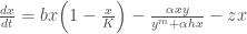

 is the prey population being harvested and
 , rather than specific parameter values,
 ![z = [z_1, z_2, ..., z_t]](https://s0.wp.com/latex.php?latex=z+%3D+%5Bz_1%2C+z_2%2C+...%2C+z_t%5D&bg=ffffff&fg=444444&s=0&c=20201002) . The process of optimizing the parameters of a state-aware control rule is known as Direct Policy Search (DPS; Quinn et al, 2017).
. The process of optimizing the parameters of a state-aware control rule is known as Direct Policy Search (DPS; Quinn et al, 2017). , is mapped to the current prey population levels,
  by the function:
![z_{t+1} = \sum_{i=1}^n w_i \Big[exp\Big[-\Big(\frac{x_t-c_i}{b_i}\Big)^2\Big]\Big]](https://s0.wp.com/latex.php?latex=z_%7Bt%2B1%7D+%3D+%5Csum_%7Bi%3D1%7D%5En+w_i+%5CBig%5Bexp%5CBig%5B-%5CBig%28%5Cfrac%7Bx_t-c_i%7D%7Bb_i%7D%5CBig%29%5E2%5CBig%5D%5CBig%5D&bg=ffffff&fg=444444&s=0&c=20201002)
 and
and  are the center, radius, and weights of each RBF
  is the number of RBFs used in the function; in this study we use
  RBFs. With two RBFs, there are a total of 6 parameters. Increasing the number of RBFs allows for more flexible function forms to be achieved. However, two RBFs have been shown to be sufficient for this problem.
![[c_1, b_1, w_1, c_2, b_2, w_2]](https://s0.wp.com/latex.php?latex=%5Bc_1%2C+b_1%2C+w_1%2C+c_2%2C+b_2%2C+w_2%5D&bg=ffffff&fg=444444&s=0&c=20201002) ), and the current prey population, to calculate the next year’s harvesting effort.
), and the current prey population, to calculate the next year’s harvesting effort. .
.![[c_1, b_1, w_1, c_2, b_2, w_2] = [0.2, 1.1, 0.41, 0.34,0.7, 0.59]](https://s0.wp.com/latex.php?latex=%5Bc_1%2C+b_1%2C+w_1%2C+c_2%2C+b_2%2C+w_2%5D+%3D+%5B0.2%2C+1.1%2C+0.41%2C+0.34%2C0.7%2C+0.59%5D+&bg=ffffff&fg=444444&s=0&c=20201002)

![c_i, b_i, w_i \in [0,1]](https://s0.wp.com/latex.php?latex=c_i%2C+b_i%2C+w_i+%5Cin+%5B0%2C1%5D&bg=ffffff&fg=444444&s=0&c=20201002) . Below is a plot of the resulting random policy functions:
. Below is a plot of the resulting random policy functions: realizations of stochasticity.
 ) is calculated as:
 is the discount rate which converts future benefits to present economic value, here
  .
.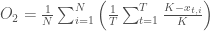


 .
.


 .
. , the historic weekly demand mean,
  , and standard deviation,
  , are applied to convert to a synthetic unit demand,
  .
.
![E[D|Q_{s_i}]](https://s0.wp.com/latex.php?latex=E%5BD%7CQ_%7Bs_i%7D%5D&bg=ffffff&fg=444444&s=0&c=20201002) , given a specific synthetic streamflow,
, given a specific synthetic streamflow,  , is:
, is:![E[D|Q_{s_i}] = E[D] + \rho \frac{\sigma_Q}{\sigma_D} (Q_i - \mu_Q)](https://s0.wp.com/latex.php?latex=E%5BD%7CQ_%7Bs_i%7D%5D+%3D+E%5BD%5D+%2B+%5Crho+%5Cfrac%7B%5Csigma_Q%7D%7B%5Csigma_D%7D+%28Q_i+-+%5Cmu_Q%29+&bg=ffffff&fg=444444&s=0&c=20201002)
 is the Pearson correlation coefficient of the weekly standardized historic inflow and demand data. Since the data is standardized, (
 ![E[d] = 0](https://s0.wp.com/latex.php?latex=E%5Bd%5D+%3D+0&bg=ffffff&fg=444444&s=0&c=20201002) and
and  ) the above form of the equation simplifies to:
![E[d|Z_{s_i}] = \rho (Z_{s_i})](https://s0.wp.com/latex.php?latex=E%5Bd%7CZ_%7Bs_i%7D%5D+%3D+%5Crho+%28Z_%7Bs_i%7D%29&bg=ffffff&fg=444444&s=0&c=20201002)
 is standard synthetic demand and
  is the standard synthetic streamflow for the
  week. The variance of the standard demand conditional upon the standard streamflow is then:
 , is then randomly sampled from a normal distribution centered around the conditional expectation with standard deviation equal to the square root of the conditional variance.
![d_{s_i} \approx N(E[d|Z_{s_i}], Var(d|Z_{s_i})^{1/2})](https://s0.wp.com/latex.php?latex=d_%7Bs_i%7D+%5Capprox+N%28E%5Bd%7CZ_%7Bs_i%7D%5D%2C+Var%28d%7CZ_%7Bs_i%7D%29%5E%7B1%2F2%7D%29&bg=ffffff&fg=444444&s=0&c=20201002)