
This semester I’m taking a Multivariate statistics course taught by Professor Scott Steinschneider in the BEE department at Cornell. I’ve been really enjoying the course thus far and thought I would share some of what we’ve covered in the class with a blog post. The material below on multicollinearity is from Dr. Steinschneider’s class, presented in my own words.
What is Multicollinearity?
Multicollinearity is the condition where two or more predictor variables in a statistical model are linearly related (Dormann et. al. 2013). The existence of multicollinearity in your data set can result in an increase of the variance of regression coefficients leading to unstable estimation of parameter values. This in turn can lead to erroneous identification of relevant predictors within a regression and detracts from a model’s ability to extrapolate beyond the range of the sample it was constructed with. In this post, I’ll explain how multicollinearity causes problems for linear regression by Ordinary Least Squares (OLS), introduce three metrics for detecting multicollinearity and detail two “Tolerant Methods” for dealing with multicollinearity within a data set.
How does multicollinearity cause problems in OLS regression?
To illustrate the problems caused by multicollinearity, let’s start with a linear regression:

Where:


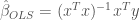
The Gauss-Markov theorem states that the Best Linear Unbiased Estimator (BLUE) for each coefficient can be found using OLS:
This estimate will have a variance defined as:
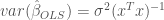
Where:

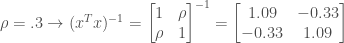
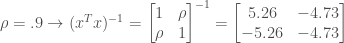
If you dive into the matrix algebra, you will find that the term (xTx) is equal to a matrix with ones on the diagonals and the pairwise Pearson’s correlation coefficients (ρ) on the off-diagonals:

As the correlation values increase, the values within (xTx)-1 also increase. Even with a low residual variance, multicollinearity can cause large increases in estimator variance. Here are a few examples of the effect of multicollinearity using a hypothetical regression with two predictors:

So why should you care about the variance of your coefficient estimators? The answer depends on what the purpose of your model is. If your only goal is to obtain an accurate measure of the predictand, the presence of multicollinearity in your predictors might not be such a problem. If, however, you are trying to identify the key predictors that effect the predictand, multicollinearity is a big problem.
OLS estimators with large variances are highly unstable, meaning that if you construct estimators from different data samples you will potentially get wildly different estimates of your coefficient values (Dormann et al. 2013). Large estimator variance also undermines the trustworthiness of hypothesis testing of the significance of coefficients. Recall that the t value used in hypothesis testing for an OLS regression coefficient is a function of the sample standard deviation (the square root of the variance) of the OLS estimator.

An estimator with an inflated standard deviation, 
Detecting Multicollinearity within a data set
Now we know how multicollinearity causes problems in our regression, but how can we tell if there is multicollinearity within a data set? There are several commonly used metrics for which basic guidelines have been developed to determine whether multicollinearity is present.
The most basic metric is the pairwise Pearson Correlation Coefficient between predictors, r. Recall from your intro statistics course that the Pearson Correlation Coefficient is a measure of the linear relationship between two variables, defined as:

A common rule of thumb is that multicollinearity may be a problem in a data set if any pairwise |r| > 0.7 (Dormann et al. 2013).
Another common metric is known as the Variance Inflation Factor (VIF). This measure is calculated by regressing each predictor on all others being used in the regression.
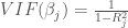
Where Rj2 is the R2 value generated by regressing predictor xj on all other predictors. Multicollinearity is thought to be a problem if VIF > 10 for any given predictor (Dormann et al. 2012).
A third metric for detecting multicollinearity in a data set is the Condition Number (CN) of the predictor matrix defined as the square root of the ratio of the largest and smallest eigenvalues in the predictor matrix:

CN> 15 indicates the possible presence of multicollinearity, while a CN > 30 indicates serious multicollinearity problems (Dormann et al. 2013).
Dealing with Multicollinearity using Tolerant Methods
In a statistical sense, there is no way to “fix” multicollinearity. However, methods have been developed to mitigate its effects. Perhaps the most effective way to remedy multicollinearity is to make a priori judgements about the relationship between predictors and remove or consolidate predictors that have known correlations. This is not always possible however, especially when the true functional forms of relationships are not known (which is often why regression is done in the first place). In this section I will explain two “Tolerant Methods” for dealing with multicollinearity.
The purpose of Tolerant Methods is to reduce the sensitivity of regression parameters to multicollinearity. This is accomplished through penalized regression. Since multicollinearity can result in large and opposite signed estimator values for correlated predictors, a penalty function is imposed to keep the value of predictors below a pre-specified value.

Where c is the predetermined value representing model complexity, p is the number of predictors and l is either 1 or 2 depending on the type of tolerant method employed (more on this below).
Ridge Regression
Ridge regression uses the L2 norm, or Euclidean distance, to constrain model coefficients (ie. l = 2 in the equation above). The coefficients created using ridge regression are defined as:

Ridge regression adds a constant, λ, to the term xTx to construct the estimator. It should be noted that both x and y should be standardized before this estimator is constructed. The Ridge regression coefficient is the result of a constrained version of the ordinary least squares optimization problem. The objective is to minimize the sum of square errors for the regression while meeting the complexity constraint.

To solve the constrained optimization, Lagrange multipliers can be employed. Let z equal the Residual Sum of Squares (RSS) to be minimized:

This can be rewritten in terms of the L2 norm of β:

Taking the derivative with respect to β and solving:


Remember that the Gauss-Markov theorem states that the OLS estimate for regression coefficients is the BLUE, so by using ridge regression, we are sacrificing some benefits of OLS estimators in order to constrain estimator variance. Estimators constructed using ridge regression are in fact biased, this can be proven by calculating the expected value of ridge regression coefficients.
![E[\hat{\beta_r}]=(I+\lambda(x^Tx)^{-1})\beta \neq \beta](https://s0.wp.com/latex.php?latex=E%5B%5Chat%7B%5Cbeta_r%7D%5D%3D%28I%2B%5Clambda%28x%5ETx%29%5E%7B-1%7D%29%5Cbeta+%5Cneq+%5Cbeta&bg=ffffff&fg=444444&s=0&c=20201002)
For a scenario with two predictors, the tradeoff between reduced model complexity and increase bias in the estimators can be visualized graphically by plotting the estimators of the two beta values against each other. The vector of beta values estimated by regression are represented as points on this plot ![(\hat{\beta}=[\beta_1, \beta_2])](https://s0.wp.com/latex.php?latex=%28%5Chat%7B%5Cbeta%7D%3D%5B%5Cbeta_1%2C+%5Cbeta_2%5D%29&bg=ffffff&fg=444444&s=0&c=20201002)


Figure 1: Geometric Interpretation of a ridge regression estimator. The blue dot indicates the OLS estimate of Beta, ellipses centered around the OLS estimates represent RSS contours for each Beta 1, Beta 2 combination (denoted on here as z from the optimization equation above). The model complexity is constrained by distance c from the origin. The ridge regression estimator of Beta is shown as the red dot, where the RSS contour meets the circle defined by c.
The c value displayed in Figure 1 is only presented to explain the theoretical underpinnings of ridge regression. In practice, c is never specified, rather, a value for λ is chosen a priori to model construction. Lambda is usually chosen through a process known as k-fold cross validation, which is accomplished through the following steps:
- Partition data set into K separate sets of equal size
- For each k = 1 …k, fit model with excluding the kth set.
- Predict for the kth set
- Calculate the cross validation error (CVerror)for kth set:
- Repeat for different values of , choose a that minimizes
![CV^{\lambda_0}_k = E[\sum(y-\hat{y})^2]](https://s0.wp.com/latex.php?latex=CV%5E%7B%5Clambda_0%7D_k+%3D+E%5B%5Csum%28y-%5Chat%7By%7D%29%5E2%5D&bg=ffffff&fg=444444&s=0&c=20201002)

Lasso Regression
Another Tolerant Method for dealing with multicollinearity known as Least Absolute Shrinkage and Selection Operator (LASSO) regression, solves the same constrained optimization problem as ridge regression, but uses the L1 norm rather than the L2 norm as a measure of complexity.
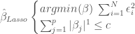
LASSO regression can be visualized similarly to ridge regression, but since c is defined by the sum of absolute values of beta, rather than sum of squares, the area it constrains is diamond shaped rather than circular. Figure 2 shows the selection of the beta estimator from LASSO regression. As you can see, the use of the L1 norm means LASSO regression selects one of the predictors and drops the other (weights it as zero). This has been argued to provide a more interpretable estimators (Tibshirani 1996).

Figure 2: Geometric interpretation of Lasso Regression Estimator. The blue dot indicates the OLS estimate of Beta, ellipses centered around the OLS estimate represents RSS contours for each Beta 1, Beta 2 combination (denoted as z from the optimization equation). The mode complexity is constrained by the L1 norm representing model complexity. The Lasso estimator of Beta is shown as the red dot, the location where the RSS contour intersects the diamond defined by c.
Final thoughts
If you’re creating a model with multiple predictors, it’s important to be cognizant of potential for multicollinearity within your data set. Tolerant methods are only one of many possible remedies for multicollinearity (other notable techniques include data clustering and Principle Component Analysis) but it’s important to remember that no known technique can truly “solve” the problem of multicollinearity. The method chosen to deal with multicollinearity should be chosen on a case to case basis and multiple methods should be employed if possible to help identify the underlying structure within the predictor data set (Dormann et. al. 2013)
Citations
Dormann, C. F., Elith, J., Bacher, S., Buchmann, C., Carl, G., Carré, G., Marquéz, J. R. G., Gruber, B., Lafourcade, B., Leitão, P. J., Münkemüller, T., McClean, C., Osborne, P. E., Reineking, B., Schröder, B., Skidmore, A. K., Zurell, D. and Lautenbach, S. 2013, “Collinearity: a review of methods to deal with it and a simulation study evaluating their performance.” Ecography, 36: 27–46. doi:10.1111/j.1600-0587.2012.07348.x
Ohlemüller, R. et al. 2008. “The coincidence of climatic and species rarity: high risk to small-range species from climate change.” Biology Letters. 4: 568 – 572.
Tibshirani, Robert 1996. “Regression shrinkage and selection via the lasso.” Journal of the Royal Statistical Society. Series B (Methodological): 267-288.

Pingback: Dealing With Multicollinearity: A Brief Overview and Introduction to Tolerant Methods | Ace Infoway
Pingback: A visual introduction to data compression through Principle Component Analysis – Water Programming: A Collaborative Research Blog
Pingback: An Introduction To Econometrics: Part 1- Classical Ordinary Least Squares Regression – Water Programming: A Collaborative Research Blog
Pingback: Water Programming Blog Guide (Part 2) – Water Programming: A Collaborative Research Blog
Pingback: Multivariate Distances: Mahalanobis vs. Euclidean – Water Programming: A Collaborative Research Blog
Pingback: From Frequentist to Bayesian Ordinary Linear Regression – Water Programming: A Collaborative Research Blog