Exploring the stability of systems of ordinary differential equations – an example using the Lotka-Volterra system of equations

Stability when dealing with dynamical systems is important
because we generally like the systems we make decisions on to be predictable.
As such, we’d like to know whether a small change in initial conditions could
lead to similar behavior. Do our solutions all tend to the same point? Would
slightly different initial conditions lead to the same or to a completely
different point for our systems.

This blogpost will consider the stability of dynamical systems of the form:

The equilibria of which are denoted by x* and y*,
respectively.

I will use the example of the Lotka-Volterra system of
equations, which is the most widely known method of modelling many predator-prey/parasite-host interactions encountered in natural systems. The Lotka-Volterra predator-prey equations were discovered independently by both Alfred Lotka and Vito Volterra in 1925-26. Volterra got to these equations while trying to explain why, immediately after WWI, the number of predatory fish was much larger than before the war.

The system is described by the following equations:

Where a, b, c, d > 0 are the parameters describing the
growth, death, and predation of the fish.

In the absence of predators, the prey population (x) grows
exponentially with an intrinsic rate of growth b.

Total predation is proportional to the abundance of prey and
the abundance of predators, at a constant predation rate a.

New predator abundance is proportional to the total
predation (axy) at a constant conversion rate c.

In the absence of prey, the predator population decreases at
a mortality rate d.

The system demonstrates an oscillating behavior, as
presented in the following figure for parameters a=1, b=1, c=2, d=1.

Volterra’s explanation for the rise in the numbers of
predatory fish was that fishing reduces the rate of increase of the prey
numbers and thus increases the rate of decrease of the predator. Fishing does
not change the interaction coefficients. So, the number of predators is
decreased by fishing and the number of prey increases as a consequence. Without
any fishing activity (during the war), the number of predators increased which
also led to a decrease in the number of prey fish.

To determine the stability of a system of this form, we
first need to estimate its equilibria, i.e. the values of x and y for which:

An obvious equilibrium exists at x=0 and y=0, which kinda
means that everything’s dead.

We’ll first look at a system that’s still alive, i.e x>0
and y>0:

And

Looking at these expressions for the equilibria we can also
see that the isoclines for zero growth for each of the species are straight
lines given by b/a for the prey and d/ca for the predator, one horizontal and
one vertical in the (x,y) plane.

In dynamical systems, the behavior of the system near an
equilibrium relates to the eigenvalues of the Jacobian (J) of F(x,y) at the equilibrium.
If the eigenvalues all have real parts that are negative, then the equilibrium
is considered to be a stable node; if the eigenvalues all have real parts that
are positive, then the equilibrium is considered to be an unstable node. In the
case of complex eigenvalues, the equilibrium is considered a focus point and
its stability is determined by the sign of the real part of the eigenvalue.

I found the following graphic from scholarpedia to be a
useful illustration of these categorizations.

So we can now evaluate the stability of our equilibria.
First we calculate the Jacobian of our system and then plug in our estimated
equilibrium.

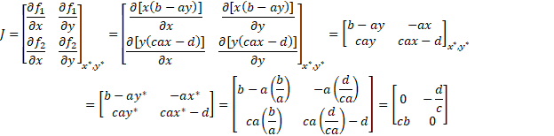
To find the eigenvalues of this matrix we need to find the
values of λ that satisfy: det⁡(J-λI)=0  where I is
the identity matrix and det denotes the determinant.

Our eigenvalues are therefore complex with their real parts equal to 0. The equilibrium is therefore a focus point, right between instability and asymptotic stability. What this means for the points that start out near the equilibrium is that they tend to both converge towards the equilibrium and away from it. The solutions of this system are therefore periodic, oscillating around the equilibrium point, with a period , with no trend either towards the
equilibrium or away from it.

One can arrive at the same conclusion by looking at the
trace (τ) of the Jacobian and its determinant (Δ).

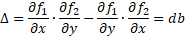
The trace is exactly zero and the determinant is positive
(both d,b>0) which puts the system right in between stability and
instability.

Now let’s look into the equilibrium where x*=0 and y*=0, aka
the total death.

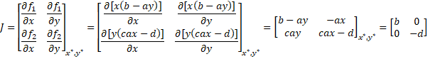
Both b and d are positive real numbers which means that the
eigenvalues will always have real values of different signs. This makes the
(0,0) an unstable saddle point. This is important because if the equilibrium of
total death were a stable point, initial low population levels would tend to
converge towards their extinction. The fact that this equilibrium is unstable
means that the dynamics of the system make it difficult to achieve total death
and that prey and predator populations could be infinitesimally close to zero
and still recover.

Now consider a system where we’ve somehow killed all the
predators (y=0). The prey would continue to grow exponentially with a growth
rate b. This is generally unrealistic for real-life systems because it assumed
infinite resources for the prey. A more realistic model would consider the prey
to exhibit a logistic growth, with a carrying capacity K. The carrying capacity of a biological species is the maximum population size of the species that can be sustained indefinitely given the necessary resources.

The model therefore becomes:

Where a, b, c, d, K > 0.

To check for this system’s stability we have to go through
the same exercise.

The predator equation has remained the same so:

For zero prey growth:

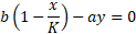
Calculating the eigenvalues becomes a tedious exercise at
this point and the time of writing is 07:35PM on a Friday. I’d rather apply a
small trick instead and use the isoclines to derive the stability of the system. The isocline for the predator zero-growth has remained the same (d/ca), which is a straight line (vertical on the (x,y) vector plane we draw before). The isocline for the prey’s zero-growth has changed to:

Which is again a straight line with a slope of –b/aK, i.e.,
it’s decreasing when moving from left to right (when the prey is increasing). Now looking at the signs in the Jacobian of the first system:

We see no self-dependence for each of the two species (the
two 0), we see that as the predator increases the prey decreases (-) and that
as the prey increases the predator increases too (+).

For our logistic growth the signs in the Jacobian change to:

Because now there’s a negative self-dependence for the prey-as its numbers increase its rate of growth decreases. This makes the trace (τ) of the Jacobian negative and the determinant positive, which implies that our system is now a stable system. Plotting the exact same dynamic system but now including a carrying capacity, we can see how the two populations converge to specific numbers.