The Reed Group Lab Manual for efficient training & open science

About a year ago, the Reed Group began to develop a group Lab Manual. The motivation of the Lab Manual is to facilitate efficient training of new students, postdocs, and collaborators on everything from basic programming and high performance computing to synthetic streamflow generation and multi-objective reservoir operations. The Lab Manual is also meant to facilitate the sharing of open science tools more broadly with other researchers and practitioners. The Lab Manual is designed to be synergistic and interactive with the Water Programming Blog, which has been advancing similar goals for 12 years and counting.

In this blog post, I will give an introductory tour of the structure and content of the Reed Group Lab Manual. This project is fully open source – you can find the lab manual hosted on GitHub Pages here, as well as the underlying code repository on GitHub here. Previous blog posts have described the technical details behind creating the lab manual with Jupyter Books and automating build and deployment with GitHub Actions, as well as detailed code snippets for two different sections of the Figure Library (post 1, post 2). The present post, on the other hand, will provide a higher level tour of the Lab Manual contents without going into code-level detail.

The Lab Manual currently contains 8 sections as laid out in the left side navigation bar: (1) Graduate Student Resources, (2) Computational Resources, (3) Software, (4) Training, (5) Water Programming Blog Post Catalog, (6) List of Paper Repositories, (7) Figure Library, and (8) Contributing to this Manual. In the remainder of this post I will give a brief overview of each section.

Graduate Student Resources

The first section is meant to provide helpful resources for new students and scholars joining the Reed Group. This includes subsections on finding housing in Ithaca and a checklist for visiting scholars. It also includes links on important courses at Cornell and conferences to consider attending. Lastly, it includes tips, resources, and templates for designing presentations, writing papers, and staying organized.

Note that a few of the resources in this section (e.g., course list, presentations) link to private resources that are only available to Reed Group members and collaborators. The rest of the site is generally designed to be fully open access.

Computational Resources

The next section is designed to bring new researchers up to speed on topics in programming, computing, and other related topics. There are pages introducing researchers to basic Python, Linux, and Git/GitHub. There are also pages on more advanced topics of machine learning, citation/reference management, high performance computing, and Python-based website deployment (such as this Lab Manual website). These pages provide some original content but also rely heavily on links to previous Water Programming Blog posts and other online resources. This section also provides access information for The Cube and Hopper, two private clusters at Cornell University that Reed Group members have access to.

Software

Next, the Software section provides information on various software tools that past and present Reed Group members have contributed to. This includes software for multi-objective evolutionary computation and exploratory modeling (Borg MOEA, Rhodium, MOEA Framework), water resources management modeling (WaterPaths, Pywr-DRB, CALFEWS), sensitivity analysis (SALib), and high-dimensional visualization (J3). Each page contains links to the software itself, along with tutorials, Water Programming Blog posts, academic papers, and other code repositories that rely on the software.

Training

The Training section satisfies a core purpose of the Lab Manual: training new students, postdocs, and collaborators on core competencies needed by Reed Group members. Topics include key methodologies that underly much of our research (e.g., MOEAs, MORDM, sensitivity analysis, scenario discovery, synthetic generation) as well as important test problems (e.g., the shallow lake problem, the fisheries game) and software (e.g., Borg MOEA, WaterPaths).

These pages build on many years of formal and informal training exercises developed by past and present Reed Group members. Each page uses a common template structure that introduces the motivation and learning objectives, the necessary software installations, the prerequisite training prior to starting the current training, and the detailed sequence of training activities ranging from literature review to model execution and analysis.

Water Programming Blog Post Catalog

To complement the training exercises in the previous section, we have also embedded a searchable table of Water Programming Blog posts within the lab manual. This allows trainees to quickly find additional helpful material that may not be directly linked to their training exercises. Note that the main page of the Blog also has its own search functionality. The search tools in the lab manual vs the blog can return different results for the same search term, so it can be helpful to try both if you are looking for posts on a particular topic.

List of Paper Repositories

The Lab Manual also contains a list of important Reed Group papers and their relevant software repositories. This can be helpful for students or other researchers who are looking to replicate or build on the workflows in those papers.

Figure Library

Next, we have a Figure Library. The purpose of this section is to facilitate collaborative development and sharing of common types of figures that Reed Group members tend to use often. As discussed in my recent blog post, there are many tools available for creating figures such as parallel coordinates plots, but they often lack the level of flexibility and detail required to create high-quality figures for presentations and papers. Thus many Reed Group members and other researchers have built their own custom visualization tools from scratch. The purpose of the Figure Library is to create a bank of such tools so that we can build off of each other’s work rather than reinventing the wheel.

Because the Lab Manual is built with Jupyter Books, each page can be built using either Markdown or Python-based Jupyter Notebooks. The latter is an excellent option for the Figure Library as it allows for seamless integration of text, code blocks, and code output such as figures.

Contributing to this Lab Manual

The last section gives detailed instructions for those who want to contribute to the Lab Manual itself. This process is fairly straightforward for those who are comfortable with basic Git-based version control. Much of the complexity of building and deploying the site is done behind the scenes using GitHub Actions and GitHub Pages each time a new commit is pushed to the Main branch of the repository. This section also provides general examples for how to build pages in Markdown and Jupyter Notebooks, as well as a template that is used to ensure consistency across Training pages. Lastly, there is an FAQ page where contributors can describe helpful fixes to problems that they have experienced when working on the Lab Manual.

Conclusion

Overall, we hope that this Lab Manual will be a valuable resource for current and future Reed Group members and collaborators. This should improve the efficiency of training new researchers while easing the burden on both trainers and trainees. In addition, we hope that it is helpful for other researchers who want to learn about our suite of methodologies and software, as well as to other research groups looking to develop their own open source lab manuals.

It is worth noting that the Reed Group Lab Manual is meant to be a living document that will continue to evolve as current and future group members contribute new content or update old content to reflect the changing state-of-the-art. What I have described in this blog post simply reflects the current iteration of this Lab Manual roughly one year from when we began this project.

Exploring time-evolving vulnerability with the newly published interactive tutorial in the Addressing Uncertainty in MultiSector Dynamics Research eBook

We recently published two new Jupyter Notebook tutorials as technical appendices to our eBook on Addressing Uncertainty in MultiSector Dynamics Research developed as part of the Integrated MultiSector, Multiscale Modeling (IM3) project, supported by the Department of Energy Office of Science’s MultiSector Dynamics Program. The eBook provides an overview of diagnostic modeling, perspectives on model evaluation, and a framework for basic methods and concepts used in sensitivity analysis. The technical appendices demonstrate key concepts introduced in the text and provide example Python code to use as a starting point for future analysis. In this post, I’ll discuss the concepts introduced in one of the new Python tutorials, Time-evolving scenario discovery for infrastructure pathways. This post will focus on the notebook’s connections to topics in the main text of the eBook rather than detailing the code demonstrated in the notebook. For details on the test case and code used in the tutorial, see the tutorial I posted last year.

In this post, I’ll first give a brief overview of the example water supply planning test case used in the tutorial, then discuss the methodological steps used to explore uncertainty and vulnerability in the system. The main topics discussed in this post are the design of experiments, factor mapping, and factor prioritization.

The Bedford-Greene water supply test case

The Bedford-Greene infrastructure investment planning problem (Figure 1) is a stylized water resources test case designed to reflect the challenges faced when evaluating infrastructure systems that evolve over time and are subject to uncertainty system inputs. The Bedford-Greene system contains two water utilities developing an infrastructure investment and management strategy to confront growing water demands and climate change. The test case was chosen for an eBook tutorial because it contains complex and evolving dynamics driven by strongly coupled human-natural system interactions. To explore these dynamics, the tutorial walks through an exploratory modeling experiment that evaluates how a large ensemble of uncertainties influences system performance and how these influences evolve over time.

In the Bedford-Greene system, modelers do not know or cannot agree upon the probability distributions of key system inputs, a condition referred to as “deep uncertainty” (Kwakkel et al., 2016). In the face of deep uncertainties, we perform an exploratory experiment to understand how a large ensemble of future scenarios may generate vulnerability for the water supply system.

Figure 1: The Bedford-Greene Water Resources Test Case

Setting up the computational experiment

The first step in the exploratory experiment is to define which factors in the mathematical model of the system are considered uncertain and how to sample the uncertainty space. The specific uncertain factors and their variability can be elicited through expert opinion, historical observation, values in literature, or physical meaning. In the Bedford-Greene system, we define 13 uncertain factors drawn from literature on real-world water supply systems (Gorelick et al., 2022). The uncertain factors used in this tutorial can be found in Table 1.

Factor Name	Plausible Range	Description
Near-Term Demand Growth Rate Mult.	-0.25 to 2.0	A scaling factor on projected demand growth over the first 15 years of the planning period
Mid-Term Demand Growth Rate Mult.	-0.25 to 2.0	A scaling factor on projected demand growth over the second 15 years of the planning period
Long-Term Demand Growth Rate Mult.	-0.25 to 2.0	A scaling factor on projected demand growth over the third15 years of the planning period
Bond Term	0.8 to 1.2	A scaling factor on the number of years over which infrastructure capital costs are repaid as debt service
Bond Interest Rate	0.6 to 1.2	A scaling factor that adjusts the fixed interest rate on bonds for infrastructure
Discount Rate	0.8 to 1.2	The rate at which infrastructure investment costs are discounted over time
Restriction Efficacy	0.8 to 1.2	A scaling factor on how effective water use restrictions are at reducing demands
Infrastructure Permitting Period	0.75 to 1.5	A scaling factor on estimated permitting periods for infrastructure projects
Infrastructure Construction Time	1 to 1.2	A scaling factor on estimated construction times for infrastructure projects
Inflow Amplitude	0.8 to 1.2	A sinusoidal scaling factor to apply non-stationary conditions to reservoir inflows
Inflow Frequency	0.2 to 0.5	A sinusoidal scaling factor to apply non-stationary conditions to reservoir inflows
Inflow Phase	-pi/2 to pi/2	A sinusoidal scaling factor to apply non-stationary conditions to reservoir inflows

Table 1: Deep Uncertainties sampled for the Bedford-Greene System

After the relevant uncertainties and their plausible ranges have been identified, the next step is to define a sampling strategy. A sampling strategy is often referred to as a design of experiments, a term that dates back to the work of Ronald Fisher in the context of laboratory or field-based experiments (Fischer, 1936). The design of experiments is a methodological choice that should be carefully considered before starting computational experiments. The design of experiments should be chosen to balance the computational cost of the exploratory experiment with the amount of information needed to accurately characterize system vulnerability. An effective design of experiments allows us to explore complex relationships within the model and evaluate the interactions of system inputs. Five commonly used designs of experiments are overviewed in Chapter 3.3 of the main text of the eBook.

In the Bedford-Greene test case, we employ a Latin Hypercube Sampling (LHS) strategy, shown in Figure 3d. With this sampling technique for the 13 factors shown in Table 1, a 13-dimensional hypercube is generated, with each factor divided into an equal number of levels to obtain 2,000 different samples of future scenarios. 2,000 samples were chosen here based on testing from similar water supply test cases (Trindade et al., 2020) for other analyses, but the sampling size must be determined on a case-by-case basis. The LHS design guarantees sampling from every level of the uncertainty space without overlaps and will generate a diverse coverage of the entire space. When the number of samples is much greater than the number of uncertain factors, LHS effectively approximates the more computationally expensive full factorial sampling scheme shown in Figure 3a without needing to constrain samples to discrete levels for each factor, as done in fractional factorial sampling, shown in Figure 3c. For more details on each sampling scheme and general information on design of experiments, see Chapter 3.3 of the eBook.

Figure 2: Alternative designs of experiments reproduced from Figure 3.3 of the eBook main text. a) full factorial design sampling of three factors at four levels with a total of 64 samples; b) the exponential growth of a necessary number of samples when applying full factorial design at four levels; c) fractional factorial design of three factors at four levels at a total of 32 samples; d) Latin Hypercube sample of three factors with uniform distributions for a total of 32 samples.

A final step in our experimental setup is to determine which model outputs are relevant to model users. In the Bedford-Greene test case, we specify five performance criteria along with performance thresholds that the water utilities would like their infrastructure investment policy to meet under all future conditions. The performance criteria and thresholds are shown in Table 2. These values are based on water supply literature, and relevant criteria and thresholds should be determined on a case-by-case basis.

Performance criteria	Threshold
Reliability	< 99%
Restriction Frequency	>20%
Worst-case cost	>10 % annual revenue
Peak financial cost	> 80% annual revenue
Stranded assets	> $5/kgal unit cost of expansion

Table 2: Performance criteria and thresholds

Discovering consequential scenarios

To explore uncertainty in the Bedford-Greene system, we run the ensemble of uncertainties developed by our design of experiments through a water resources systems model and examine the outputs of each sampled combination of uncertainty. In this system, we’re interested in understanding 1) which uncertainties have the most impact on system vulnerability, 2) which combinations of uncertainties lead to consequential outcomes for the water supply system, and 3) how vulnerability evolves over time. Chapter 3.2 of the eBook introduces diagnostic approaches that can help us answer these questions. In this tutorial, we utilize gradient-boosted trees, a machine-learning algorithm that uses an ensemble of shallow trees to generate an accurate classifier (for more on boosting, see Bernardo’s post). Gradient-boosted trees are particularly well suited to infrastructure investment problems because they are able to capture non-linear and non-differential boundaries in the uncertainty space, which often occur as a result of discrete capacity expansions. Gradient-boosted trees are also resistant to overfitting, easy to interpret, and provide a simple means of ranking the importance of uncertainties. For more background on gradient-boosted trees for scenario discovery, see this post from last year.

Gradient-boosted trees provide a helpful measure of feature importance, the percentage decrease in the impurity of the ensemble of trees associated with each factor. We can use this measure to examine how each uncertainty contributes to the ability of the region’s infrastructure investment and management policy. Infrastructure investments fundamentally alter the water utilities’ storage-to-capacity ratios and levels of debt burden, which will impact their vulnerability over time. To account for these changes, we examine feature importance over three different time periods. The results of our exploratory modeling process are shown in Figure 3. We observe that the importance of various uncertainties evolves over time for both water utilities. For example, while near-term demand growth is a key factor for both utilities in all three time periods, restriction effectiveness is a key uncertainty for Bedford in the near- and mid-term but not in the long-term, likely indicating that infrastructure investment reduces the utility’s need to rely on water use restrictions. Greene is not sensitive to restriction effectiveness in the near-term or long-term, but is very sensitive in the mid-term. This likely indicates that the utility uses restrictions as a bridge to manage high demands before infrastructure investments have been fully constructed.

Figure 3: factor importance for the two utilities. Darker colors indicate that uncertainties have higher predictive value for discovering consequential scenarios.

To learn more about how vulnerability for the two water utilities evolves, we use factor mapping (eBook Chapter 3.2) to delineate regions of the uncertainty space that lead to consequential model outputs. The factor maps in Figures 4 and 5 complement the factor ranking in Figure 3 by providing additional information about which combinations of uncertainties generate vulnerability for the two utilities. While near-term demand growth and restriction effectiveness appear to generate vulnerability for Bedford in the near-term, Figure 4 reveals that the vast majority of sampled future states of the world meet the performance criteria. When evaluated using a 22-year planning horizon, however, failures emerge as a consequence of high demand and low restriction effectiveness. When evaluated across a 45-year planning horizon, the utility appears extremely vulnerable to high demand, indicating that the infrastructure investment policy is likely insufficient to maintain water supply reliability.

Figure 4: Factor maps for Bedford

Greene’s factor maps tell a different story. In the near-term, the utility is vulnerable to high-demand scenarios. In the mid-term, the vulnerable regions have transformed, and two failure modes are apparent. First, the utility is vulnerable to a combination of high near-term demand and low restriction effectiveness, indicating the potential for water supply reliability failures. Second, the utility is vulnerable to low-demand scenarios, highlighting a potential financial failure from over-investment in infrastructure. When analyzed across the 45-year planning horizon, the utility is vulnerable to only low-demand futures, indicating a severe financial risk from over-investment. These factor maps provide important context to the factor priorities shown in Figure 3. While the factor prioritization does highlight the importance of demand growth for Greene, it does not indicate which ranges of uncertainty generate vulnerability. Evaluating the system across time reveals that though the utility is always sensitive to demand growth, the consequences of demand growth and the range that generates vulnerability completely transform over the planning period.

Figure 5: Factor maps for Greene

Concluding thoughts

The purpose of this post was to provide additional context to the eBook tutorial on time-evolving scenario discovery. The Bedford-Greene test case was chosen because it represents a tightly coupled human natural system with complex and nonlinear dynamics. The infrastructure investments made by the two water utilities fundamentally alter the system’s state dynamics over time, necessitating an approach that can capture how vulnerability evolves. Through a carefully designed computational experiment, and scenario discovery using gradient-boosted trees, we discover multiple failure modes for both water utilities, which can help regional decision-makers monitor policy performance and adapt to changing conditions. While each application will be different, the code in this tutorial can be used as a starting point for applying this methodology to other human-natural systems. As with all tutorials in the eBook, the Jupyter notebook ends with a section on how to apply this methodology to your problem.

References

Kwakkel, J. H., Walker, W. E., & Haasnoot, M. (2016). Coping with the wickedness of public policy problems: approaches for decision making under deep uncertainty. Journal of Water Resources Planning and Management, 142(3), 01816001.

Fisher, R.A. (1936). Design of experiments. Br Med J, 1(3923):554–554

Trindade, B. C., Gold, D. F., Reed, P. M., Zeff, H. B., & Characklis, G. W. (2020). Water pathways: An open source stochastic simulation system for integrated water supply portfolio management and infrastructure investment planning. Environmental Modelling & Software, 132, 104772.

Creating a collaborative lab manual pt. 2: Automated build & deploy with GitHub Actions

In my last blog post, I introduced the collaborative lab manual that the Reed Group is beginning to develop. Although the content of this site is still very much a work in progress, the goal is for this lab manual to help streamline the process of onboarding new students, postdocs, and collaborators by acting as a centralized location for readings, training materials, and coding resources relevant to our group’s research. As described in the previous post, the site itself is built using the Jupyter Books package for Python, which allows for Markdown documents and executable Jupyter Notebooks to be translated into static HTML websites.

However, the distributed nature of this project, with multiple collaborators developing material for the site from their own computers, initially led to some software dependency challenges. As the project has evolved, we have worked to overcome these challenges using GitHub Actions. This post will describe our GitHub Actions workflow, which automatically rebuilds the site in a consistent way after each new update, without inheriting specific software dependencies from individual developers, and then automatically deploys the updated site using GitHub Pages. All code used to build and deploy the lab manual can be found in this GitHub repository.

GitHub Actions workflow

This post will build on Travis Thurber’s previous blogpost on Continuous Integration/Continuous Delivery (CI/CD), GitHub Actions, and GitHub Pages, so I would recommend checking that out first if you have not already. As discussed in that post, GitHub Actions are automated processes that can be triggered by particular events within a GitHub repository (e.g., updates to the code base). The instructions for executing these processes are written in a YAML script, .github/workflows/deploy.yml. GitHub automatically looks for scripts in this directory to trigger automated GitHub Actions.

### github actions to build & deploy book, following https://github.com/executablebooks/cookiecutter-jupyter-book/blob/main/.github/workflows/deploy.yml

name: deploy

on:
  # Trigger the deploy on push to main branch
  push:
    branches:
      - main
  schedule:
    # jupyter-book is updated regularly, let's run this deployment every month in case something fails
    # <minute [0,59]> <hour [0,23]> <day of the month [1,31]> <month of the year [1,12]> <day of the week [0,6]>
    # https://pubs.opengroup.org/onlinepubs/9699919799/utilities/crontab.html#tag_20_25_07
    # https://crontab.guru/every-month
    # Run cron job every month
    - cron: '0 0 1 * *'

jobs: 
  # This job deploys the example book
  deploy-example-book:
    runs-on: ${{ matrix.os }}
    strategy:
      matrix:
        os: [ubuntu-latest]
        python-version: [3.8]
    steps:
    - uses: actions/checkout@v2

    # Install python
    - name: Set up Python ${{ matrix.python-version }}
      uses: actions/setup-python@v1
      with:
        python-version: ${{ matrix.python-version }}

    # install virtual environment with caching, so only updates when requirements.txt changes,
    # based on https://github.com/marketplace/actions/restore-or-create-a-python-virtualenv#custom_virtualenv_dir
    # Note: virtual environment by default will be created under ~/.venv
    - uses: syphar/restore-virtualenv@v1
      id: cache-virtualenv
      with:
        requirement_files: docs/requirements_py.txt
    - uses: syphar/restore-pip-download-cache@v1
      if: steps.cache-virtualenv.outputs.cache-hit != 'true'

    # install python dependencies    
    - name: Install python dependencies
      run: pip install -r docs/requirements_py.txt
      if: steps.cache-virtualenv.outputs.cache-hit != 'true'

    # update kernel of all jupyter notebooks to .venv to match GH action environment
    - name: Update Jupyter Notebook kernels 
      run: python docs/update_jupyter_kernels.py .venv |
           python -m ipykernel install --user --name=.venv

    # install R
    - name: Install R
      uses: r-lib/actions/setup-r@v2
      with:
        use-public-rspm: true
    # install R dependencies
    - name: Install R dependencies
      run: sh docs/install_R_dependencies.sh

    # Build the example book
    - name: Build book
      run: jupyter-book build --all docs/

    # Deploy html to gh-pages
    - name: GitHub Pages action
      uses: peaceiris/actions-gh-pages@v3.6.1
      with:
        github_token: ${{ secrets.GITHUB_TOKEN }}
        publish_dir: docs/_build/html
        publish_branch: gh-pages

I borrowed initially from the example Jupyter Books deployment that can be found here. This Action (Line 3) has a number of steps, which will be outlined sequentially. First, in Lines 5-16, we establish the set of conditions that trigger automated execution of the Action: (1) the Action will be triggered each time an update is pushed to the main branch of the repository; and (2) the Action will be triggered on the first of each month, regardless of whether any new updates have been pushed to the repository, which should help ensure that software dependencies remain up to date over time.

Next, in Lines 18-27, we specify that the Action should be executed on an Ubuntu virtual machine (latest available version). In Lines 29-48, we instruct the Action to install Python 3.8 on the virtual machine, and then install all Python packages listed in the file docs/requirements_py.txt. Standardizing the operating system and software dependencies using a virtual machine, as opposed to building and deploying locally on individual developers’ machines, helps to avoid situations wherein one developer accidentally breaks functionality introduced by another developer due to differences in their local software environments.

One downside to rebuilding a new virtual machine each time the Action is run is that this can be rather slow, especially for complicated software environments, e.g., those with many Python package installations. However, one way to make this process more efficient is to create a virtual environment which can be cached and reloaded into memory. This process is implemented in Lines 35-48, using the restore_virtualenv “task” in the GitHub Action Marketplace. Now the Python environment will only need to be rebuilt when the requirements_py.txt file has changed since the last commit; otherwise, the cached virtual environment can be loaded from memory in order to save time.

Another issue we encountered relates to the naming of virtual environments within Jupyter Notebooks. When you create a new Notebook on a personal computer, you will generally need to specify the Python “Kernel” manually using the graphical user interface. The Kernel can either be the generic Python interpreter you have installed (e.g., Python 3.8), or else a specific virtual environment that you have installed for a particular purpose (e.g., .venv_spatial). Once you have selected a Kernel, the Notebook will expect the same Kernel to be available as the default whenever the Notebook is run. This can cause errors when working on teams where different contributors have different naming conventions for their environments. For example, consider a situation where Contributor A develops a Jupyter Notebook-based page on spatial analysis, using the local virtual environment .venv_spatial. Contributor B then pulls Contributor A’s changes, including the new Notebook on spatial analysis, and then adds her own new Notebook on machine learning using the environment .venv_ML. When Contributer B tries to build the Jupyter Book (more on this process later), the spatial analysis notebook will exit with an error saying that the .venv_spatial environment cannot be found. Contributer B could manually change the Notebook Kernel to .venv_ML or another local environment, but this is not an ideal solution for long-term collaborative interoperability. To circumvent this issue, Lines 50-53 execute the script docs/update_jupyter_kernels.py:

### script to update the kernel for all Jupyter notebooks to user-specified name, given as argv
### this will be run by GitHub Action to set Kernel to .venv before deploying website. Can also be run by user if their env has different name.

import glob
import json
import sys

venv_name = sys.argv[1]
nbpaths = glob.glob('*.ipynb') + glob.glob('*/*.ipynb') + glob.glob('*/*/*.ipynb')

for nbpath in nbpaths:
    ### load jupyter notebook into dict based on its json format
    with open(nbpath) as f:
        nbdict = json.load(f)
    ### update kernel metadata
    nbdict['metadata']['kernelspec']['display_name'] = venv_name
    nbdict['metadata']['kernelspec']['name'] = venv_name
    ### write updated dict to json/ipynb
    with open(nbpath, 'w') as f:
        json.dump(nbdict, f, indent=2)

The purpose of this Python script is to reassign all Jupyter Notebooks within the repository to use the same Kernel name, .venv (supplied as a command line argument). The key insight is that Jupyter Notebooks are actually stored on disc in structured JSON format (try opening one in a text editor to verify this). The script above leverages this fact to programmatically replace the existing Kernel name with our new name, .venv. By running this command in GitHub Actions, we can automatically standardize the Kernel for all Notebooks to use the virtual environment that we created in Lines 35-48 (.venv is the default environment name used by the restore_virtualenv task). Note that this should not impact the Kernel names in the repository itself, since this script is only being run on the GitHub Actions virtual machine. However, if individual contributors experience local errors from incompatible Kernel names, they can either change the Kernel manually in the Notebook GUI (the old fashion way), or else run the update_jupyter_kernels.py script on their own machine with their unique Python virtual environment name given as a command line argument.

Returning to the deploy.yml file, the next step is to install the R programming language (Lines 55-59) and any necessary R libraries (Lines 60-62). The latter step is accomplished by running the script docs/install_R_dependencies.sh.

#!/bin/bash
### script for installing R dependencies from requirements file
### simplified version of code here: https://stackoverflow.com/questions/54534153/install-r-packages-from-requirements-txt-files
while IFS=" " read -r package;
do
        Rscript -e "install.packages('"$package"')";
done < "docs/requirements_r.txt"

This Bash script reads a list of dependencies from the file docs/requirements_r.txt and installs each library on top of the base R installation on our virtual machine. Unfortunately the R installations are quite slow, but I am not aware of any virtual environment caching task for R on GitHub Actions.

Returning again to the deploy.yml file, the next step in Lines 64-66 is to build the static HTML site using the Jupyter Books functionality. The command in Line 66 ( jupyter-book build --all docs/ ) is also the command used to build a site locally when individual contributors want to test their work before pushing changes to the main repository. In this case, this command will create a separate folder of HTML files which can be opened in a browser.

However, when running on the virtual machine through GitHub Actions, the new HTML files are not yet being hosted anywhere. The final set of commands in Lines 68-74 accomplish this by restructuring and organizing the file contents on the virtual machine (including the new HTML files) to match the structure that is expected by GitHub Pages. The updated files are then committed and pushed to a separate branch of the GitHub repository called gh-pages. This gh-pages branch should only be altered by GitHub Actions, as opposed to being developed directly by humans like the main branch.

Finally, because gh-pages is set as the source branch for our GitHub Pages site, the updates pushed to this branch by the GitHub Action will automatically deploy the updated HTML files to our lab manual webpage.

To verify that all of these steps on the virtual machine completed successfully, we can check the Action log on GitHub. This shows that each step completed as expected without errors, along with the time to complete each step. If errors do occur, each of these steps can be expanded to show the errors and other terminal outputs in more detail.

Overall, this workflow based on GitHub Actions is helping us to streamline our processes for collaborative development of a group lab manual. Our hope is that this workflow will continue to adapt over time based on our evolving needs, much like the living document of the lab manual itself.

Creating a collaborative research group lab manual with Jupyter Books

Motivation

Onboarding new students, staff, or collaborators can be a challenge in highly technical fields. Often, the knowledge needed to run complex experiments or computing workflows is spread across multiple individuals or teams based on their unique experiences, and training of new team members tends to occur in an ad hoc and inefficient manner. These challenges are compounded by the inevitable turnover of students, postdocs, and external collaborators in academic research settings.

Over the years, the Reed Group has developed a large bank of training materials to help streamline the onboarding process for new team members. These materials introduce concepts and tools related to water systems modeling, multi-objective evolutionary algorithms, global sensitivity analysis, synthetic streamflow generation, etc. However, these materials are still spread across a variety of sources (academic papers, GitHub repositories, blog posts, etc.) and team members, and there has been growing recognition of the need to catalogue and compile relevant resources and trainings in a more structured way.

For this reason, we have begun to create a lab manual for the Reed group. This will include a wide variety of information relevant to new students and researchers – everything from training exercises and code snippets, to reading lists and coursework suggestions, to a code of conduct outlining our values and expectations. The goal is for this to be a collaborative, living document created and maintained by students and postdocs. Ideally this will continue to evolve for years along with the evolving state-of-the-art in methodology, software, and literature.

After considering a number of different platforms for constructing websites, we settled on the Jupyter Book package for Python. You can find our lab manual here, and the source code used to create it here – note that this is still very much in development, a skeleton waiting to be fleshed out. In the remainder of this blog post, I will highlight the major elements of a Jupyter Book website, using our skeleton lab manual as an example. Then in a future blog post, I will outline the Continuous Integration and Continuous Delivery (CI/CD) strategy we are using to manage versioning and platform dependency issues across multiple developers.

Intro to Jupyter Book

Jupyter Book is a Python package for creating static websites. The package is built on the popular Sphinx engine used to create documentation for many of your favorite Python packages. Sphinx was also used to create the ebook for “Addressing Uncertainty in MultiSector Dynamics Research“, as described in two recent blog posts by Rohini Gupta and Travis Thurber. The ebook was a source of inspiration for our lab manual and the reason we initially considered Sphinx-based workflows. However, Jupyter Books layers several additional functionalities on top of Sphinx. First, it supports use of the MyST Markdown language, which is more familiar and intuitive to most researchers than the reStructured Text format favored by Sphinx. And second, it allows for pages to be built from executable Jupyter Notebooks, a powerful tool for combining text and equations with formatted code blocks, program output, and generated figures.

The Jupyter Book documentation contains tutorials, examples, and references, and is an excellent resource for anyone looking to build their own site. The documentation itself is, of course, created using the Jupyter Book package, and interested readers can check out the source code here.

Designing the website structure

The hierarchical structure of a Jupyter Book is defined in a simple YAML-style Table of Contents file, which should be named _toc.yml. Here is the TOC for our lab manual at present:

format: jb-book
root: intro.md
parts:
- chapters:
  - file: ExamplePages/ExamplePages.md
    sections:
    - file: ExamplePages/mdExample.md
    - file: ExamplePages/nbExample.ipynb
  - file: Resources/Resources.md
    sections:
    - file: Resources/ClusterBasics.md
    - file: Resources/Computing.md
    - file: Resources/Courses.md
    - file: Resources/DataVisualization.md
    - file: Resources/LifeAtCornell.md
    - file: Resources/ReedGroupTools.md
    - file: Resources/WritingProcess.md
    - file: Resources/CitationNetworkandDiscovery.md
  - file: Training/Training.md
    sections:
    - file: Training/Schedule.md
    - file: Training/Reading.md
    - file: Training/LakeProblem.md
    - file: Training/Training_Fisheries_Part1.md
    - file: Training/Linux_MOEAs_HPC.md

The “root” defines the landing page, in this case the intro.md markdown file. That landing page will link to three “chapters” called ExamplePages, Resources, and Training. Each of these chapters has it’s own landing page as well as multiple child “sections.” Each page can either be written as a Markdown file (.md) or a Jupyter Notebook (.ipynb).

The other important YAML file for all Jupyter Books is _config.yml:

title: Reed group lab manual
author: The Reed Group at Cornell CEE
logo: logo.png

# Force re-execution of notebooks on each build.
# See https://jupyterbook.org/content/execute.html
execute:
  execute_notebooks: force

# Define the name of the latex output file for PDF builds
latex:
  latex_documents:
    targetname: book.tex

# Add a bibtex file so that we can create citations
bibtex_bibfiles:
  - references.bib

# Information about where the book exists on the web
repository:
  url: https://github.com/reedgroup/reedgroup.github.io  # Online location of your book
  path_to_book: docs  # Optional path to your book, relative to the repository root

# Add GitHub buttons to your book
# See https://jupyterbook.org/customize/config.html#add-a-link-to-your-repository
html:
  use_issues_button: true
  use_repository_button: true

We first define our website’s title and author, as well as an image logo to display. The line “execute_notebooks: force” means that we want to reexecute all Jupyter Notebooks each time the site is built (see docs for other options). The url gives the web address where we want to host our site – in this case the GitHub Pages address associated with the GitHub repository for the site. The path_to_book defines “docs” as the folder in the repository where all source code is to be held. Finally, the last two options are used to create buttons at the top of our site that link to the GitHub repository in case readers want to browse the source code or report an issue. For now, we are using the default vanilla style, but there are many ways to customize the structural and aesthetic style of the site. You would need to point to custom style files from this configuration file – see the Jupyter Book gallery for inspiration.

Building pages with Markdown and Jupyter Notebooks

Jupyter Book makes it very easy to write new pages using either Markdown or Jupyter Notebooks. For context, here is a screenshot of the site’s homepage:

The main content section for this page is built from the “root” file, intro.md:

# Welcome to our lab manual! 

```{warning}
This site is still under construction
```

The purpose of this site is to help new students and collaborators get up to speed on the research methods/tools used by the Reed Group. This page is designed and maintained by other graduate students and post docs, and is intended to serve as a living document. 

This manual was created using the Jupyter Books Python package, and is hosted with GitHub Pages. You can find our source code at https://github.com/reedgroup/reedgroup.github.io.

```{tableofcontents}```

As you can see, this uses a very human-readable and intuitive Markdown-based file structure. Jupyter Book provides simple functionality for warning labels and other emphasis boxes, as well as a Table of Contents that is automatically rendered from the _toc.yml file. The tableofcontents command can be used from anywhere in the hierarchical page tree and will automatically filter to include only children of the current page. The separate sidebar TOC will also expand to show “sections” as you navigate into different “chapters.” For example, here is the Markdown and rendered webpage for the “ExamplePages” chapter:

# Example Pages with JupyterBooks
```{tableofcontents}```

For more detailed pages, you can also apply standard Markdown syntax to add section headers, bold/italic font, code blocks, lists, Latex equations, images, etc. For example, here is ExamplePages/mdExample.md:

# Markdown example
This is an example page using just markdown

### Subsection 1
Here is a subsection

### Subsection 2
Here is another subsection. 

:::{note}
Here is a note!
:::

And here is a code block:

```
e = mc^2
```

And here comes a cute image!

![capybara and friends](capybaraFriends.jpg "Capybara and friends")

Lastly, and most importantly for purposes of building a training manual, we can create pages using Jupyter Notebooks. For example, here are two screenshots of the webpage rendered from ExamplePages/nbExample.ipynb:

As you can see, the Notebook functionality allows us to combine text and equations with rendered Python code. We can also execute Bash, R, or other programs using Jupyter Notebook’s “magic” commands. Note that the Jupyter-based website is not interactive – for that you’ll need Binder, as demonstrated in this blog post by David Gold.

Nevertheless, the Notebook is reexecuted each time we rebuild the website, which should really streamline collaborative lab manual development. For example, once we have developed a code bank of visualization examples (stay tuned!), it will be straightforward to edit the existing examples and/or add new examples, with the rendered visualizations being automatically updated rather than needing to manually upload the new images. Additionally, reexecuting the Notebooks each time we rebuild the site will force us to maintain the functionality of our existing code bank rather than letting portions become obsolete due to package dependencies or other issues.

Next steps

You now have the basic building blocks to create your own lab manual or ebook using a collection of YAML files, Markdown files, and Jupyter Notebooks. The last two critical steps are to actually build the static site (e.g., the html files) using Jupyter Book, and then host the site using GitHub pages. I will demonstrate these steps, as well as our CI/CD strategy based on GitHub Actions, in my next blog post.

Fisheries Training 0: Exploring Predator-Prey Dynamics

Hello there, welcome to a new training series!

In a series of five posts, we will be analyzing and exploring the Fisheries Game, which is a rich, predator-prey system with complex and nonlinear dynamics arising from the interactions between two fish species. This game will be used to walk through the steps of performing a broad a posteriori decision making process, including the exploration and characterization of impacts of system uncertain on the performance outcomes. It also serves as a conceptual tool to demonstrate the importance of accounting for deep uncertainty, and the significance of its effects on system response to management actions.

A GitHub repository containing all of the necessary code for this series is available here, and will be updated as the series develops.

We will begin here (Post 0) with an introduction to the Fisheries Game, using a modified form of the Lotka-Volterra equations for predator-prey dynamics.

Toward the end of this post, we will provide an overview of where this series is going and the tools that will be used along the way.

A very quick introduction to the Lotka-Volterra system of equations

In this game, we are stakeholders for a managed fishery. Our goal is to determine a harvesting strategy which balances tradeoffs between ecological and economic objectives. Throughout this process we will consider ecological stability, harvest yield, harvest predictability, and profits while attempting to maintain the robustness of both the ecological system and economic performance under the presence of uncertainty.

The first step in our decision making process is to model population dynamics of the fish species.

Equation 1: The base Lotka-Volterra SOE.

Equation 1 is the original Lotka-Volterra system of equations (SOE) as developed independently by Alfred Lotka in 1910, and by Vito Volterra in 1928. In this equation, x is the population density of the prey, and y is the population density of the predator. This SOE characterizes a prey-dependent predator-prey functional response, which assumes a linear relationship between prey consumption and predator growth.

Arditi and Akçakaya (1990) constructed an alternative predator-prey SOE, which assume a non-linear functional response (i.e., predator population growth is not linear with consumption). It accounts for predation efficiency parameters such as interference between predators, time needed to consume prey after capture, and a measure of how long it takes to convert consumed prey into new predators. This more complex SOE takes the form:

Equation 2: The full predator-dependent predator-prey SOE, including predator interference (m) and harvesting (z).

The full description of the variables are as follows: x and y are the prey and predator population densities at time t respectively (where t is in years); α is the rate at which the predator encounters the prey; b is the prey growth rate; c is the rate at which the predator converts prey to new predators; d is predator death rate; h is the time it needs to consume the prey (handling time); K is the environmental carrying capacity; m is the level of predator interaction; and z is the fraction of the prey population that is harvested. In this post, we will spend some time exploring the potential behavior of these equations.

Before proceeding further, here are some key terms used throughout this post:

• Zero isoclines: Lines on the plot indicating prey or predator population levels that result in constant population size over time (zero growth rate).
• Global attractor: The specific value that the system tends to evolve toward, independent of initial conditions.
• Equilibrium point: The intersection of two (or more) zero isoclines; a point or line of trajectory convergence.
  • Stable (nontrivial) equilibrium: Equilibrium at which both prey and predator exist
  • Unstable equilibrium: Global attractor is a stable limit cycle
• Stable limit cycle: A closed (circular) trajectory
• Trajectory: The path taken by the system given a specific set of initial conditions.
• Functional response: The rate of prey consumption by your average predator.

Population equilibrium and stability

When beginning to consider a harvesting policy, it is important to first understand the natural stability of the system.

Population equilibrium is a necessary condition for stability. The predator and prey populations are in equilibrium if the rate of change of the populations is zero:

Predator stability

Let’s first consider the equilibria of the predator population. In this case, we are only interested in the non-trivial (or co-existence) equilibria where the predator and prey populations are non-zero (, and ).

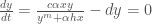
Here, we are interested in solving for the predator zero-isocline () which satisfies this equation. Re-arrangement of the above equation yields:

Solving for yields the predator zero-isocline:

In the context of the fisheries, we are interested in the co-existence conditions in which . From the zero-isocline stability equation above, it is clear that this is only true if:

Simply put, the rate at which predators convert prey into new predators () must be greater than the death rate () scaled by the time it needs to consume prey ().

Prey stability

A similar process can be followed for the derivation of the zero-isocline stability condition for the prey population. The stability condition can be determined by solving for:

As the derivation of the prey isocline is slightly more convoluted than the predator isocline, the details are not presented here, but are available in the Supplementary Materials of Hadjimichael et al. (2020), which is included in the GitHub repository for this post here.

Resolution of this stability condition yields the second necessary co-existence equilibrium condition:

Uncertainty

As indicated by the two conditions above, the stability of the predator and prey populations depends upon ecosystem properties (e.g., the availability of prey, , predator interference, , and the carrying capacity, ), unique species characteristics (e.g., the prey growth rate, , and predation efficiency parameters , ).

Specification of different values for these parameters results in wildly different system dynamics. Below are examples of three different population trajectories, each generated using the same predator-dependent system of equations, with different parameter values.

Figure 1: Three trajectory fields, resulting from predator-prey models with different parameter values. (a) A stable equilibrium with a single global attractor (values: a = 0.01, b = 0.35, c = 0.60, d = 0.20, h = 0.44, K = 1900, m = 0.30, z = 0.0); (b) an unstable system with limit cycles as global attractors (values: a = 0.32, b = 0.48, c = 0.40, d = 0.16, h = 0.23, K = 2400, m = 0.30, z = 0.0); (c) an unstable system with deterministic extinction of both species (values: a = 0.61, b = 0.11, c = 0.80, = 0.18, h = 0.18, K = 3100, m = 0.70, z = 0.0).

Exploring system dynamics (interactive!)

To emphasize the significance of parameter uncertainty on the behavior of predator-prey system behavior, we have prepared an interactive Jupyter Notebook. Here, you have ability to interactively change system parameter values and observe the subsequent change in system behavior.

The Binder link to the interactive Jupyter Notebook prepared by Trevor Amestoy can be found here. Before the code can be run, open the ‘Terminal’, as shown in Figure 2 below.

Figure 2: Starting page of the Jupyter Notebook binder.

Install the necessary libraries by entering the following line into the terminal:

pip install numpy scipy matplotlib pandas

You’re good to go once the libraries have been loaded. Open the Part_0_Interactive_fisheries_ODEs.ipynb file in the Part_0_ODE_Dynamics/ folder.

Play around with the sliders to see what system trajectories you end up with! Notice how abruptly the population dynamics change, even with minor changes in parameter values.

The following GIFs show some potential trajectories you might observe as you vary the ranges of the variables:

Starting at a stable equilibrium

In Figure 3 below, both prey and predator eventually coexist at constant population sizes with no human harvesting.

Figure 3: The Fisheries system at a stable equilibrium quickly transitioning to an unstable equilibrium, and back again to a stable equilibrium.

However, this is a fishery with very small initial initial prey population size. Here, note how quickly the system changes from one of stable equilibrium into that of unstable equilibrium with a small decrease in the value of α. Without this information, stakeholders might unintentionally over-harvest the system, causing the extinction of the prey population.

Starting at an unstable equilibrium

Next, Figure 4 below shows an unstable equilibrium with limit cycles and no human harvesting.

Figure 4: An unstable equilibrium where the both prey and predator populations oscillate in a stable limit cycle.

Figure 4 shows that a system will be in a state of unstable equilibrium when it takes very little time for the predator to consume prey, given moderately low prey population sizes and prey population growth rate. Although predators die at a relatively high rate, the prey population still experiences extinction as it is unable to replace population members lost through consumption by the predator species. This is a system in which stakeholders might instead choose to harvest the predator species.

Introducing human harvesting

Finally, a stable equilibrium that changes when human harvesting of the prey population is introduced in Figure 5 below.

Figure 5: An unstable equilibrium where the both prey and predator populations oscillate in a stable limit cycle.

This Figure demonstrates a combination of system parameters that might represent a system that can be harvested in moderation. It’s low prey availability is abated by a relatively high predator growth rate and relatively low conversion rates. Be that as it may, exceeding harvesting rates may suddenly cause the system to transition into an unstable equilibrium, or in the worst case lead to an unexpected collapse of the population toward extinction.

Given that the ecosystem parameters are uncertain, and that small changes in the assumed parameter values can result in wildly different population dynamics, it begs the question: how can fisheries managers decide how much to harvest from the system, while maintaining sustainable population levels and avoiding system collapse?

This is the motivating question for the upcoming series!

The MSD UC eBook

To discover economic and environmental tradeoffs within the system, reveal the variables shaping the trajectories shown in Figure 3 to 5, and map regions of system vulnerability, we will need suitable tools.

In this training series, we will be primarily be using the MSD UC eBook and its companion GitHub repository as the main resources for such tools. Titled ‘Addressing uncertainty in MultiSector Dynamics Research‘, the eBook is part of an effort towards providing an open, ‘living’ toolkit of uncertainty characterization methods developed by and for the MultiSector Dynamics (MSD) community. The eBook also provides a hands-on Jupyter Notebook-based tutorial for performing a preliminary exploration of the dynamics within the Fisheries Game, which we will be expanding on in this tutorial series. We will primarily be using the eBook to introduce you to sensitivity analysis (SA) methods such as Sobol SA, sampling techniques such as Latin Hypercube Sampling, scenario discovery approaches like Logistic Regression, and their applications to complex, nonlinear problems within unpredictable system trajectories. We will also be making frequent use of the functions and software packages available on the MSD GitHub repository.

To make the most out of this training series, we highly recommend familiarizing yourself with the eBook prior to proceeding. In each of the following posts, we will also be making frequent references to sections of the eBook that are relevant to the current post.

Training sequence

In this post, we have provided an overview of the Fisheries Game. First, we introduced the basic Lotka-Volterra equations and its predator-dependent predator-prey variation (Arditi and Akcakaya, 1990) used in Hadjimichael et al. (2020). We also visualized the system and explored how the system trajectories change with different parameter specifications. Next, we introduced the MSD UC eBook as a toolkit for exploring the Fisheries’ system dynamics.

Overall, this post is meant to be a gateway into a deep dive into the system dynamics of the Fisheries Game as formulated in Hadjimichael et al. (2020), using methods from the UC eBook as exploratory tools. The next few posts will set up the Fisheries Game and its objectives for optimization, explore the implications of varying significant decision variables, map parameter ranges that result in system vulnerability, and visualize these outcomes. The order for these posts are as follows:

Post 1 Problem formulation and optimization of the Fisheries Game in Rhodium

Post 2 Visualizing and exploring the Fisheries’ Pareto set and Pareto front using Rhodium and J3

Post 3 Identifying important system variables using different sensitivity analysis methods

Post 4 Mapping consequential scenarios that drive the Fisheries’ vulnerability to deep uncertainty

That’s all from us – see you in Post 1!

References

Abrams, P., & Ginzburg, L. (2000). The nature of predation: prey dependent, ratio dependent or neither?. Trends In Ecology &Amp; Evolution, 15(8), 337-341. https://doi.org/10.1016/s0169-5347(00)01908-x

Arditi, R., & Akçakaya, H. R. (1990). Underestimation of Mutual Interference of Predators. Oecologia, 83(3), 358–361. http://www.jstor.org/stable/4219345

Hadjimichael, A., Reed, P., & Quinn, J. (2020). Navigating Deeply Uncertain Tradeoffs in Harvested Predator-Prey Systems. Complexity, 2020, 1-18. https://doi.org/10.1155/2020/4170453

Lotka, A. (1910). Contribution to the Theory of Periodic Reactions. The Journal Of Physical Chemistry, 14(3), 271-274. https://doi.org/10.1021/j150111a004

Reed, P.M., Hadjimichael, A., Malek, K., Karimi, T., Vernon, C.R., Srikrishnan, V., Gupta, R.S., Gold, D.F., Lee, B., Keller, K., Thurber, T.B, & Rice, J.S. (2022). Addressing Uncertainty in Multisector Dynamics Research [Book]. Zenodo. https://doi.org/10.5281/zenodo.6110623

Volterra, V. (1928). Variations and Fluctuations of the Number of Individuals in Animal Species living together. ICES Journal Of Marine Science, 3(1), 3-51. https://doi.org/10.1093/icesjms/3.1.3

Make your Git repository interactive with Binder

Have you ever tried to demo a piece of software you wrote only to have the majority of participants get stuck when trying to configure their computational environment? Difficulty replicating computational environments can prevent effective demonstration or distribution of even simple codes. Luckily, new tools are emerging that automate this process for us. This post will focus on Binder, a tool for creating custom computing environments that can be distributed and used by many remote users simultaneously. Binder is language agnostic tool, and can be used to create custom environments for R, Python and Julia. Binder is powered by BinderHub, an open source service in the cloud. At the bottom of this post, I’ll provide an example of an interactive Python Jupyter Notebook that I created using BinderHub.

BinderHub

BinderHub combines two useful libraries: repo2docker and JupyterHub. repo2docker is a tool to build, run and push Docker images from source code repositories. This allows you to create copies of custom environments that users can replicate on any machine. These copies are can be stored and distributed along with the remote repository. JuptyerHub is a scalable system that can be used to spawn multiple Jupyter Notebook servers. JuptyerHub takes the Docker image created by repo2docker and uses it to spawn a Jupyter Notebook server on the cloud. This server can be accessed and run by multiple users at once. By combining repo2docker and JupyterHub, BinderHub allows users to both replicate complex environments and easily distribute code to large numbers of users.

Creating your own BinderHub deployment

Creating your own BinderHub deployment is incredibly easy. To start, you need a remote repository containing two things: (1) a Jupyter notebook with supporting code and (2) configuration files for your environment. Configuration files can either be an environment.yml file (a standard configuration file that can be generated with conda, see example here) or a requirements.txt file (a simple text file that lists dependencies, see example here).

To create an interactive BinderHub deployment:

1. Push your code to a remote repository (for example Github)
2. Go to mybinder.org and paste the repository’s URL into the dialoge box (make sure to select the proper hosting service)
3. Specify the branch if you are not on the Master
4. Click “Launch”

The website will generate a URL that you can copy and share with users. I’ve created an example for our Rhodium tutorial, which you can find here:

https://mybinder.org/v2/gh/dgoldri25/Rhodium/master?filepath=DMDU_Rhodium_Demo.ipynb

To run the interactive Jupyter Notebook, click on the file titled “Rhodium_Demo.ipynb”. Happy sharing!

Introducing Julia: A Fast and Modern Language

In this blog post, I am introducing Julia, a high-level open-source dynamic programming language. While it has taken root in finance, machine learning, life sciences, energy, optimization, and economic realms, it is certainly not common within the water programming realm. Through this post, I will give an overview of the features, pros, and cons of Julia before comparing its performance to Python. Following this, I give an overview of common Julia development environments as well as linking to additional resources.

Julia: What’s Going On?

Julia is a high-level open-source dynamic programming language built for scientific computing and data processing that is Pythonic in syntax to ensure accessibility while boosting computational efficiency.  It is parallelizable on high performance computing resources utilizing CPUs and GPUs, allowing for its use in large-scale experiments.

With Version 1.1.0 recently released, Julia now stands amongst the established and stable programming languages. As such, Julia can handle matrices with ease while performing at speeds nearly comparable to C and Fortran. It is comparable to Cython/Numba and faster than Numpy, Python, Matlab, and R. Note that further benchmarking is required on a project-specific basis due to the speed of individual packages/libraries, but a simple case is shown in the following section.

The biggest case for implementing Julia over C/C++/Fortran is its simplicity in writing and implementation. Its language is similar Python, allowing for not only list comprehension but also ‘sloppy’ dynamic variable type declarations and use. Julia has the ability to move between dynamic and static variable types. Furthermore, Julia allows users to create unique variable types, allowing for maximum flexibility while maintaining efficiency.

Installing and implementing packages from the start is nearly seamless, simply requiring the name of the package and an internet connection. Most packages and libraries are hosted on GitHub and are relatively straightforward to install with just a couple lines of code. On the same hand, distributing and contributing to the opensource community is straightforward. Furthermore, Julia can access Python modules with wrappers and C/Fortran functions without, making it a very versatile language. Likewise, it can easily be called from Python (PyJulia) to speed up otherwise cumbersome operations.

Julia has relatively straightforward profiling modules built in. Beyond being able to utilize Jupyter Notebook commands, Julia has a range of code diagnostic tools, such as a @Time command to inform the user of wall time and memory allocation for a function.

One of the most obvious downsides to Julia when compared to Python is the relatively small community. There is not nearly the base of documentation that I am accustomed to; nearly every issue imaginable in the Python world has been explored on Stack Overflow, Julia is much more limited. However, because much of its functionality is based on MATLAB, similar issues and their corresponding solutions bleed over.

Additional transition issues that may be encountered is that unlike Python, Julia’s indexing begins with 1. Furthermore, Julia uses column-major ordering (like Matlab, Fortran, and R) unlike Python and C (row-major ordering), making iterating column-by-column substantially faster. Thus, special care must be taken when switching between languages in addition to ensuring consistent strategies for speeding up code. Another substantial transition that may be required is that Julia is not directly object-oriented since objects do not directly have embedded methods; instead, a given object must be passed to a function to be modified.

Overall, I see Julia as having the potential to improve computational efficiency for computationally-intensive models without the need to learn a more complex language (e.g. Fortran or C/C++). Between its ease of integration between other common languages/libraries to its ability to properly utilize HPC CPU/GPU resources, Julia may be a useful tool to utilize alongside Python to create more efficient large-scale models.

Julia Allows for Faster Matrix Operations

As a simple test to compare scalability of Julia and Python, I computed the dot product of increasingly large matrices using the base Julia language and Numpy in Python (both running in Jupyter Notebooks on a Windows desktop). You can find the code at the following link on Github.

As you can see in the generated figure, Julia outperforms Python for large matrix applications, indicating that Julia is more efficient and may be worth using for larger and larger operations. If you have any suggestions on improving this code for comparison, please let me know; I am absolutely game for improvement.

Development Environments for Julia

The first and most obvious variables on what development environment is best is you, the user. If you’re wanting all the bells and whistles versus a simple text-editing environment, the range of products to fulfill you desires exists.

Juno—an extension to Atom—is the default IDE that is incorporated with JuliaPro, a pre-packaged version of Julia that includes a range of standard packages—Anaconda is the parallel in the Python world.

Jupyter Notebooks  are my go-to development environment for experimenting with code in both Python and Julia, especially for testing small sections of code.  Between being able to easily create visuals and examples inline with your code and combining code with Markdown, it allows for clean and interactive approach to sharing code or teaching. Note that installation generally requires IJulia but can allow for easy integration into already existing Jupyter workflows.

JetBrains IDEs (e.g. CLion, PyCharm) support a Julia plugin that supports a wide range of the same features JetBrains is known for. However, it is still in beta and is working to improve its formatter and debugging capabilities.

JuliaBox is an online web interface using Jupyter Notebooks for code development on a remote server, requiring no local installation of Julia. Whether you are in a classroom setting, wanting to write code on your phone, or are just wanting to experiment with parallel computing (or don’t have access to HPC resources), JuliaBox allows for a nearly seamless setup experience. However, note that this development environment limits each session to 90 minutes (up to 8 hours on a paid subscription) and requires a subscription to access any resources beyond 3 CPU cores. Note that you can access GPU instances with a paid subscription.

Julia Studio is a default IDE used by a range of users. It is a no-frills IDE based on Qt Creator, resulting in a clean look.

For anyone looking to use Visual Studio, you can install a VS Code extension.

Vim is not surprisingly available for Julia.  And if you’re feeling up the challenge, Emacs also has an interface.

Of course, you can just use a texteditor of your choice (e.g. Sublime Text with an extension) and simply run Julia from the terminal.

Julia Resources

• Installing Julia
• Julia’s wide range of learning resources
• Learn Julia the Hard Way
• Julia Style Guide
• Trending Julia Packages
• Stable (and standard) Julia Packages
• Julia Code Profiling Guide
• PyPlots in Julia
• Calling Python Functions in Julia 
• Weave, a Report Generator: Made for Julia, Weave incorporates languages including Markdown, Pandoc, and LaTex to generate reports. It integrates with IJulia to work with Jupyter Notebooks
• Julia Subreddit Community

Acknowledgements

Thanks to Dave Gold for his assistance in giving guidance for benchmarking and reminding me of the KISS principle.

Launching Jupyter Notebook Using an Icon/Shortcut in the Current Working Directory Folder

A petty annoyance I’ve encountered when wanting to open Jupyter Notebook (overview) is that I couldn’t find a way to instantly open it in my current Windows Explorer window. While one trick you can use to open the Command Prompt in this folder is by typing ‘cmd’ in the navigation bar above (shown below) and pressing Enter/Return, I wanted to create a shortcut or icon I could double-click in any given folder and have it open Jupyter Notebook in that same working directory.

This method allows you to drag-and-drop the icon you create into any folder and have it launch Jupyter Notebook from the new folder. It works for Windows 7, 8, and 10. Please feel free to let me know if you encounter any errors!

A great application for this shortcut may be to include this shortcut in GitHub folders where you wish to direct someone to launch Jupyter Notebook with minimal confusion. Just direct them to double-click on the icon and away they go!

Creating Your Own Jupyter Notebook Shortcut

To begin, we must have already installed Jupyter Notebook or Jupyter Lab. Next, navigate to the folder we want to create your shortcut. Right-click, select ‘New’, then create a shortcut. 

In the Create Shortcut Windows prompt, type the location of the item you want the Shortcut Icon to direct to. In this case, we are wanting direct this shortcut to the Command Prompt and have it run the command to open Jupyter Notebook. Copy/paste or type the following into the prompt:

cmd /k “jupyter notebook”

Note that cmd will change to the location of the Command Prompt executable file (e.g. C:\Windows\System32\cmd.exe), and ‘/k’ keeps the Command Prompt window open to ensure Jypyter Notebook does not crash. You can edit the command in the quotation marks to any command you would want, but in this case ‘jupyter notebook’ launches an instance of Jupyter Notebook.

You can then save this shortcut with whatever name you wish!

At this point, double-clicking the shortcut will open Jupyter Notebook in a static default directory (e.g. ‘C:\Windows\system32’). To fix this, we need to ensure that this shortcut instead directs to the current working directory (the location of the shortcut).

Next, we need to edit the location where the Command Prompt will run in. Right-click on your newly-created icon and select ‘Properties’ at the bottom of the menu to open the window shown on the left. One thing to note is that the ‘Target’ input is where we initially put in our ‘location’ prompt from above.

At this point, change the ‘Start in:’ input (e.g. ‘C:\Windows\system32’) to the following:

%cd%

By changing this input, instead of starting the Command Prompt in a static default directory, it instead starts the command prompt  in the current working directory for the shortcut.

At this point, you’re finished! You can drag and drop this icon to any new folder and have Jupyter Notebook start in that new folder.

If you wish to download a copy of the shortcut from Dropbox. Note that for security reasons, most browsers, hosting services, and email services will rename the file from ‘jupyter_notebook_shortcut.lnk’ to ‘jupyter_notebook_shortcut.downloads’.

Many thanks to users on superuser for helping develop this solution!

Please let me know if you have any questions, comments, or additional suggestions on applications for this shortcut!

 

Jupyter Notebook: A “Hello World” Overview

Jupyter Notebook: Overview

When first learning Python, I was introduced to Jupyter Notebook as an extremely effective IDE for group-learning situations. I’ve since used this browser-based interactive shell for homework assignments, data exploration and visualization, and data processing. The functionality of Jupyter Notebook extends well past simple development and showcasing of code as it can be used with almost any Python library (except for animated figures right before a deadline). Jupyter Notebook is my go-to tool when I am writing code on the go.

As a Jupyter Notebook martyr, I must point out that Jupyter Notebooks can be used for almost anything imaginable. It is great for code-oriented presentations that allow for running live code, timing of lines of code and other magic functions, or even just sifting through data for processing and visualization. Furthermore, if documented properly, Jupyter Notebook can be used as an easy guide for stepping people through lessons. For example, check out the structure of this standalone tutorial for NumPy—download and open it in Jupyter Notebook for the full experience. In a classroom setting, Jupyter Notebook can utilize nbgrader to create quizzes and assignments that can be automatically graded. Alas, I am still trying to figure out how to make it iron my shirt.

A Sample Jupyter Notebook Presentation (credit: Matthew Speck)

One feature of Jupyter Notebook is that it can be used for a web application on a server-client structure to allow for users to interact remotely via ssh or http. In an example is shown here, you can run Julia on this website even if it is not installed locally. Furthermore, you can use the Jupyter Notebook Viewer to share notebooks online.  However, I have not yet delved into these areas as of yet.

For folks familiar with Python libraries through the years, Jupyter Notebook evolved from IPython and has overtaken its niche. Notably, it can be used for over 40 languages—the original intent was to create an interface for Julia, Python and R, hence Ju-Pyt-R— including Python, R, C++, and more. However, I have only used it for Python and each notebook kernel will run in a single native language (although untested workaround exist).

Installing and Opening the Jupyter Notebook Dashboard

While Jupyter Notebook comes standard with Anaconda, you can easily install it via pip or by checking out this link.

As for opening and running Jupyter Notebook, navigate to the directory (in this case, I created a directory in my username folder titled ‘Example’) you want to work out of in your terminal (e.g. Command Prompt in Windows, Terminal in MacOS) and run the command ‘jupyter notebook’.

Opening the Command Prompt

Once run, the following lines appear in your terminal but are relatively unimportant. The most important part is being patient and waiting for it to open in your default web browser—all mainstream web browsers are supported, but I personally use Chrome.

 

 

Opening Jupyter Notebook on Windows

Opening Jupyter Notebook on MacOS

If at any time you want to exit Jupyter Notebook, press Ctrl + C twice in your terminal to immediately shut down all running kernels (Windows and MacOS). Note that more than one instance of Jupyter Notebook can be running by utilizing multiple terminals.

Creating a Notebook

Once Jupyter Notebook opens in your browser, you will encounter the dashboard. All files and subdirectories will be visible on this page and can generally be opened or examined.

Initial Notebook Dashboard Without Any Files

If you want to create a shiny new Notebook to work in, click on ‘New’ and select a new Notebook in the language of your choice (shown below). In this case, only Python 3 has been installed and is the only option available. Find other language kernels here.

Opening a New Notebook

Basic Operations in Jupyter Notebook

Once opened, you will find an untitled workbook without a title or text. To edit the title, simply left-click on ‘Untitled’ and enter your name of choice.

Blank Jupyter Notebook

To write code, it is the same as writing a regular Python script in any given text editor. You can divide your code into separate sections that are run independently instead of running the entire script again. However, when importing libraries and later using them, you must run the corresponding lines to import them prior to using the aforementioned libraries.

To run code, simply press Shift + Enter while the carat—the blinking text cursor—is in the cell.

Jupyter Notebook with Basic Operations

After running any code through a notebook, the file is automatically backed up in a hidden folder in your working directory. Note that you cannot directly open the notebook (IPYNB File) by double-clicking on the file. Rather, you must reopen Jupyter Notebook and access it through the dashboard.

Directory where Sample Jupyter Notebook Has Been Running

As shown below, you can easily generate and graph data in line. This is very useful when wanting to visualize data in addition to modifying a graphic (e.g. changing labels or colors). These graphics are not rendered at the same DPI as a saved image or GUI window by default but can be changed by modifying matplotlib’s rcParams.

Example Histogram in Jupyter Notebook

Conclusion

At this point, there are plenty of directions you can proceed. I would highly suggest exploring some of the widgets available which include interesting interactive visualizations. I plan to explore further applications in future posts, so please feel free to give me a yell if you have any ideas.