Welcome to Water Programming! This blog is by Pat Reed’s group at Cornell, who use computer programs to solve problems — Multiobjective Evolutionary Algorithms (MOEAs), simulation models, visualization, and other techniques. Use the search feature and categories on the right panel to find topics of interest. Feel free to comment, and contact us if you want to contribute posts.
The MOEAFramework Setup Guide: A detailed guide is now available. The focus of the document is connecting an optimization problem written in C/C++ to MOEAFramework, which is written in Java.
The Borg MOEA Guide: We are currently writing a tutorial on how to use the C version of the Borg MOEA, which is being released to researchers here.
Call for contributors: We want this to be a community resource to share tips and tricks. Are you interested in contributing? Please email Lillian Lau at lbl59@cornell.edu. You’ll need a WordPress.com account.
This blog post details the available information from Colorado state’s decision tools that can be used in different research areas. These tools have extensive information on water administration, climate data, reservoir details, and groundwater data. Snapshots of each tool are provided to highlight the features.
Prior Appropriation Doctrine is the priority system followed. Water source, location structure, call priority, and priority date details are accessible. Administrative call data is also available (active and historical). The following is the snapshot of viewing active call data. The additional resources tab in the lower bottom has more information linking to call analysis for each structure and water source. Acquisition and new appropriation data for lakes and streams is also available. Decree details, court docs and net amounts for different structure types (acquifer reservation, augmentation plan, basin determination, ditch system, entity, erosion control dam, exchange plan, livestock water tank, measuring point, Mine, minimum flow, pipeline, power plant, pump, reach and recharge area) can be accessed in https://dwr.state.co.us/Tools/WaterRights/NetAmounts
Climate data is available for 12157 stations from different sources such as NRCS, NOAA, CoCoRaHS, and CoAgMet. The data can be viewed as a table, or graph and downloaded as a CSV file for each site. Climate parameters include evaporation, temperature, precipitation, snow, vapor pressure and wind speed.
Information on the structural details of the dam is provided under the dam safety tool. The data can be downloaded from this link. Data includes 53 columns for each dam with details on dam type, length, height, crest elevation, storage, federal regulations, surface area, drainage area, spillway capacity, outlet description, last inspection date, safe storage and others.
This page has well-documented groundwater level reports for the years 1989-2023 for aquifers in different basins of the Colorado state along with rules for water well construction and inspection details. The groundwater – water levels tool has data for around 10000 wells with details on well name, water level depth, water level elevation, period of record count, measured agency, aquifer name, county, basin and others. Well permit data is available in this page.
Current and historical gage data is available for 2554 stations with tabled data on station name, station type, data source, river source, record start date and end date. This page has the details on stream gage station, diversion structures and storage structures. Along with flow data, different environmental variables data is available as water temperature, air temperature, conductivity, pH.
GIS data is available for download for all river basins that includes different layers as diversion, wells, streams/rivers, canals, irrigated acreage and climate stations. Other tools include location converter and distance calculator (https://dwr.state.co.us/Tools/Home). They also provide an extensive tool called Map Viewer that can be used to view GIS data online. Different map viewers are as follows
Map Description
Link
DWR Map Viewer: All inclusive map viewer with over 170 map layers of DWR and CWCB data. (Use the Layer Catalog to add layers that are not pre-populated.)
CWCB Data Viewer: View data specific to CWCB instream flows, Construction Fund loans, recreational in-channel diversions (RICDs), WSRF grants and more.
This flow tool is built for ecological risk assessment in the basin. This tool is developed in excel and has embedded historical and future datasets of colorado river basin. Future data is available for five planning scenarios defined as business as casual, weak economy, cooperative growth, adaptive innovation and hot growth. Environmental flow risk categories are low, moderate, less moderate, high and very high ecological risk. Ecological risk maps are generated for each basin.
CWCB released update to water plan for use by researchers, decision makers, water users and stakeholders with data on historical and future availability covering different sectors utilizing the above defined tools. In my opinion, this report is worth reading to understand the Colorado’s water assessment.
All the heading are linked to web pages where the tool data is available which are accessible as of May 6, 2024.
In this blog post, we will be reviewing how to perform runtime diagnostics using MOEAFramework. This software has been used in prior blog posts by Rohini and Jazmin to perform MOEA diagnostics across multiple MOEA parameterizations. Since then, MOEAFramework has undergone a number of updates and structure changes. This blog post will walk through the updated functionality of running MOEAFramework (version 4.0) via the command line to perform runtime diagnostics across 20 seeds using one set of parameters. We will be using the classic 3-objective DTLZ2 problem optimized using NSGAII, both of which are in-built into MOEAFramework.
Before we begin, some helpful tips and system configuration requirements:
Ensure that you have the latest version of Java installed (as of April 2024, this is Java Version 22). The current version of MOEAFramework was compiled using class file version 61.0, which was made available in Java Version 17 (find the complete list of Java versions and their associated class files here). This is the minimum requirement for being able to run MOEAFramework.
The following commands are written for a Linux interface. Download a Unix terminal emulator like Cygwin if needed.
Another helpful tip: to see all available flags and their corresponding variables, you can use the following structure:
For the a full list of parameter files for each of the in-built MOEAFramework algorithms, please see Jazmin’s post here.
In this example, I have called it NSGAII_Params.txt. Note that maxEvaluations is set to 10,000 on both its lower and upper bounds. This is because we want to fix the number of function evaluations completed by NSGAII. Next, in our command line, we run:
The output NSGAII_Latin file should contain a single-line that can be opened as a text file. It should have six tab-delineated values that correspond to the six parameters in the input file that you have generated. Now that you have your MOEA parameter files, let’s begin running some optimizations!
First, make a new folder in your current directory to store your output data. Here, I am simply calling it data.
mkdir data
Next, optimize the DTLZ2 3-objective problem using NSGAII:
for i in {1..20}; do java -cp MOEAFramework-4.0-Demo.jar org.moeaframework.analysis.tools.RuntimeEvaluator --parameterFile NSGAII_Params.txt --input NSGAII_Latin --problem DTLZ2_3 --seed $i --frequency 1000 --algorithm NSGAII --output data/NSGAII_DTLZ2_3_$i.data; done
Here’s what’s going down:
First, you are performing a runtime evaluation of the optimization of the 3-objective DTLZ2 problem using NSGAII
You are obtaining the decision variables and objective values at every 1,000 function evaluations, effectively tracking the progress of NSGAII as it attempts to solve the problem
Finally, you are storing the output in the data/ folder
You then repeat this for 20 seeds (or for as many as you so desire).
Double check your .data file. It should contain information on your decision variables and objective values at every 1,000 NFEs or so, seperated from the next thousand by a “#”.
Generate the reference set
Next, obtain the only the objective values at every 1,000 NFEs by entering the following into your command line:
for i in {1..20}; do java -cp MOEAFramework-4.0-Demo.jar org.moeaframework.analysis.tools.ResultFileMerger --problem DTLZ2_3 --output data/NSGAII_DTLZ2_3_$i.set --epsilon 0.01,0.01,0.01 data/NSGAII_DTLZ2_3_$i.data; done
Notice that we have a new flag here – the --epsilon flag tells MOEAFramework that you only want objective values that are at least 0.01 better than other non-dominated objective values for a given objective. This helps to trim down the size of the final reference set (coming up soon) and remove solutions that are only marginally better (and may not be decision-relevant in the real-world context).
On to generating the reference set – let’s combine all objectives across all seeds using the following command line directive:
for i in {1..20}; do java -cp MOEAFramework-4.0-Demo.jar org.moeaframework.analysis.tools.ReferenceSetMerger --output data/NSGAII_DTLZ2_3.ref -epsilon 0.01,0.01,0.01 data/NSGAII_DTLZ2_3_$i.set; done
Your final reference set should now be contained within the NSGAII_DTLZ2_3.ref file in the data/ folder.
Generate the runtime metrics
Finally, let’s generate the runtime metrics. To avoid any mix-ups, let’s create a folder to store these files:
mkdir data_metrics
And finally, generate our metrics!
or i in {1..20}; do java -cp MOEAFramework-4.0-Demo.jar org.moeaframework.analysis.tools.ResultFileEvaluator --problem DTLZ2_3 --epsilon 0.01,0.01,0.01 --input data/NSGAII_DTLZ2_3_$i.data --reference data/NSGAII_DTLZ2_3.ref --output data_metrics/NSGAII_DTLZ2_3_$i.metrics; done
If all goes well, you should see 20 files (one each for each seed) similar in structure to the one below in your data_metrics/ folder:
The header values are the names of each of the MOEA performance metrics that MOEAFramework measures. In this blog post, we will proceed with visualizing the hypervolume over time across all 20 seeds.
Visualizing runtime diagnostics
The following Python code first extracts the metric that you would like to view, and saves the plot as a PNG file in the data_metrics/ folder:
If you correctly implemented the code, you should be able to be view the following figure that shows how the hypervolume attained by the NSGAII algorithm improves steadily over time.
In the figure above, the colored inner region spans the hypervolume attained across all 20 seeds, with the dotted line representing the mean hypervolume over time. The solid upper and lower bounding lines are the maximum and minimum hypervolume achieved every 1,000 NFEs respectively. Note that, in this specific instance, NSGAII only achieves about 50% of the total hypervolume of the overall objective space. This implies that a higher NFE (a longer runtime) is required for NSGAII to further increase the hypervolume achieved. Nonetheless, the rate of hypervolume increase is gradually decreasing, indicating that this particular parameterization of NSGAII is fast approaching its maximum possible hypervolume, which additional NFEs only contributing small improvements to performance. It is also worth noting the narrow range of hypervolume values, especially as the number of NFEs grows larger. This is representative of the reliability of the NGSAII algorithm, demonstrating that is can somewhat reliably reproduce results across multiple different seeds.
Summary
This just about brings us to the end of this blog post! We’ve covered how to perform MOEA runtime diagnostics and plot the results. If you are curious, here are some additional things to explore:
Plot different performance metrics against NFE. Please see Joe Kasprzyk’s post here to better understand the plots you generate.
Explore different MOEAs that are built into MOEAFramework to see how they perform across multiple seeds.
Generate multiple MOEA parameter samples using the in-built MOEAFramework Latin Hypercube Sampler to analyze the sensitivity of a given MOEA to its parameterization.
Attempt examining the runtime diagnostics of Borg MOEA using the updated version of MOEAFramework.
On that note, make sure to check back for updates as MOEAFramework is being actively reviewed and improved! You can view the documentation of Version 4.0 here and access its GitHub repository here.
‘Does the flap of a butterfly’s wing in Brazil stir up a tornado in Texas?’ These words reflect the so-called ‘butterfly effect’ typically ascribed to Edward Lorenz (MIT), who was a pioneer in the field of numerical weather prediction (NWP). (Interestingly, Lorenz himself first referred to the ‘flap of a seagulls’ wing’; the butterfly swap out was the work of a creative conference session convener. Somewhat coincidentally, the shape of the ‘Lorenz attractor’ is also reminiscent of a butterfly, see Figure 1). Motivated by the very salient challenge in the post-WWII era to improve weather prediction capabilities for strategic purposes, he developed a theoretical framework for the predictability of non-linear dynamical systems in a seminal paper, ‘Deterministic nonperiodic flow’ (Lorenz, 1963), that would come to be known as ‘chaos theory’ or ‘chaotic dynamics’. This theory was foundational to the development of ensemble forecasting (and a whole host of other things), and still underpins our current theoretical understanding of the inherent predictability of complex dynamical systems like the atmosphere (Lorenz, 2006).
Figure 1. Book cover (left panel) and the characteristic ‘butterfly wing’ shape of the Lorenz attractor (right panel) from his seminal 1963 work. (Palmer, 1993)
In actuality, the whole ‘flap of a butterfly’s wing creating a tornado in Texas’ relates specifically to only one aspect of the theoretical framework developed by Lorenz. In this post, I will attempt to give a slightly fuller treatment of this theoretical framework and its development. My hope is that this post will be a theoretical primer for two follow-on practically oriented posts: 1) a discussion of the state-of-the-science of hydrometeorological ensemble forecasting and its application in emerging water resources management practices like forecast informed reservoir operations, and 2) a deeper dive into ensemble verification techniques. While the techniques for (2) are grounded in the theoretical statistical properties of stochastic-dynamic predictive ensembles, they have broad applications to any scenario where one needs to diagnose the performance of an ensemble.
The Lorenz model and ‘chaos’ theory
When most people hear the word ‘chaos’, they tend to think of the dictionary definition: ‘complete disorder and confusion’ (Oxford), which in a scientific context might aptly describe some sort of white noise process. As you will see, this is somewhat of a far cry from the ‘chaos’ described in Lorenz’s theory. The ‘chaos’ terminology was actually coined by a later paper building on Lorenz’s work (Li & Yorke, 1975) and as noted by Wilks (2019): ‘…this label is somewhat unfortunate in that it is not really descriptive of the sensitive-dependence phenomenon’. The sensitive-dependence phenomenon is one of a set of 4 key properties (to be discussed later) that characterize the behaviors of the sort of non-linear, non-periodic deterministic systems that Lorenz argued were most representative of the atmosphere. In contrast to ‘disorder’ and ‘confusion’, these properties, in fact, lend some sense of order to the evolution of these dynamical systems, although the nature of that order is highly dependent on the system state.
A deterministic, non-periodic systems model
First, let’s dive into a few details of Lorenz’s 1963 work, using some figures and descriptions from a later paper (Palmer, 1993) that are easier to follow. While the 1963 paper is quite dense, much of the mathematical logic is dedicated to justifying the use of a particular system of equations that forms the basis of the study. This system of 3 equations and 3 variables (X, Y, Z) describes a non-linear, dissipative model of convection in a fluid of uniform depth, where there is a temperature difference between the upper and lower surfaces. Lorenz derived the set of 3 equations shown in the upper left panel of Figure 2 from earlier work by Rayleigh (1916) on this particular problem. In short, X relates to the intensity of convective motion, Y relates to the temperature difference between ascending and descending currents, and Z relates to the distortion of the vertical temperature profile from linearity; the details of these variables are not actually all that important to the study. What is important is that this system of equations has no general solutions (aside from the steady state solution) and must be numerically integrated in the time dimension to determine the convective flow dynamics. The ‘trajectories’ of these integrations shown in the phase space diagrams in Figure 2 exhibit the sorts of unstable, non-periodic behaviors that Lorenz thought were the most useful analog to atmospheric dynamics, albeit in a much simpler system. (‘Much’ is an understatement here; modern NWP models have a phase space on the order of 109 in contrast to the 3-dimensional phase space of this problem, Wilks, 2019. Of note, the use of phase-space diagrams (i.e. plots where each axis corresponds to a dependent variable in the system of equations) preceded Lorenz, but his use of them is perhaps one of the best-known early instances of this kind of visualization. Other uses of phase space relationships can be found in Rohini’s post or Dave’s post)
Figure 2. a) Lorenz equations and the XY phase space diagram of their integrations. b-c) X variable timeseries of two separate integrations of the Lorenz equations from very similar initial conditions. (Palmer, 1993)
Regime structure and multiple distinct timescales
What ‘behaviors’ then, are we talking about? Referring again to Figure 2a, we see the projection of a long series of model integration trajectories onto the XY-plane of the phase space diagram, where each dot is a timestep in the integration. What is immediately apparent in the form of these integrations is the two lobed ‘butterfly’ shape of the diagram. Each lobe has a central attractor where the trajectories often reside for multiple revolutions, but can then transition to the other attractor when passing near the center of the diagram. These so-called ‘Lorenz attractors’ comprise one of the key properties of chaotic dynamics, namely regime structure, which is tendency of the trajectories to reside around phase space attractors for some period of time. This residence time in a regime is generally quite a bit longer than the timescales of the trajectories’ individual revolutions around an attractor. This attribute is referred to as multiple distinct timescales and is evidenced in Figure 2b-c, where smaller amplitude sections of the timeseries show residence in one or the other regime and large amplitude sections describe transitions between regimes. Often, but not always, the residence in these regimes occurs for multiple revolutions, suggesting that there are shorter timescale evolutions of the system that take place within these regimes, while infrequent, random shifts to the other regimes occur at longer timescales.
Sensitive-dependence and state-dependent variation in predictability
Figure 3. a-c) Different trajectories through the XY phase space dependent on the initial condition state-space (black circle). (Palmer, 1993)
Returning now to the ‘butterfly effect’; what, then, is this whole sensitive-dependence thing mentioned earlier? Figure 3a-c provide a nice graphical representation of this phenomenon. In each panel, a set of nearby initial states are chosen at different location in the phase space diagram and then are followed through their set of trajectories. In 3a, these trajectories neatly transition from one regime to the other, remaining relatively close to each other at the trajectories’ end. In 3b, a set of initial states not so far from 3a are chosen and instead of neatly transitioning to the other regime, they diverge strongly near the center of the diagram, with some trajectories remaining in the original regime, and some transitioning. However, for about half of the timespan, the trajectories remain very close to one another. Finally, an initial state chosen near the center of the diagram (3c) diverges quickly into both regimes, with trajectories ending up at nearly opposite ends of the phase space (black tails at upper right and left of diagram). Figures b-c, in particular, showcase the sensitive-dependence on initial conditions attributes of the system. In other words, from a set of very close-by initial states, the final trajectories in phase space can yield strongly divergent results. Importantly, this divergence in trajectories over some period of time can occur right away (3c), at some intermediate time (3b), or not at all (3a).
This is the basic idea behind the last core property of these systems, state-dependent variation in predictability. Clearly, a forecast initialized from the starting point in 3a could be a little bit uncertain about the exact starting state and still end up in about the right spot for an accurate future prediction at the end of the forecast horizon. At medium ranges, this is also the case for 3b, but the longer range forecast is highly uncertain. For 3c, all forecast ranges are highly uncertain; in other words, the flap of a butterfly’s wing can mean the difference between one or the other trajectory! Importantly, one can imagine in this representation that an average value of 3c’s trajectories (i.e. the ensemble mean) would fall somewhere in the middle of the phase space and be representative of none of the two physically plausible trajectories into the right or left regimes. This is an important point that we’ll return to at the end of this post.
From the Lorenz model to ensemble forecasting
The previous sections have highlighted this idealized dynamical system (Lorenz model) that theoretically has properties of the actual atmosphere. Those 4 properties (the big 4!) were: 1) sensitive-dependence on initial conditions, 2) regime structure, 3) multiple distinct timescales, and 4) state-dependent variation in predictability. In this last section, I will tie these concepts into a theoretical discussion of ensemble forecasting. Notably, in the previous sections, I discussed ‘timescales’ without any reference to the real atmosphere. The dynamics of the Lorenz system prove to be quite illuminating about the actual atmosphere when timescales are attached to the system that are roughly on the order of the evolution of synoptic scale weather systems. If one assumes that a lap around the Lorenz attractor equates to a synoptic timescale of ~5 days, then the Lorenz model can be conceptualized in terms of relatively homogenous synoptic weather progressions occurring within two distinct weather regimes that typically persist on the order of weeks to months (see Figure 3b-c). This theoretical foundation jives nicely with the empirically derived weather-regime based approach (see Rohini’s post or Nasser’s post) where incidentally, 4 or more weather regimes are commonly found (The real atmosphere is quite a bit more complex than the Lorenz model after all). This discussion of the Lorenz model has hopefully given you some intuition that conceptualizing real world weather progressions outside the context of an appropriate regime structure could lead to some very unphysical representations of the climate system.
Ensemble forecasting as a discrete approximation of forecast uncertainty
In terms of weather prediction, though, the big 4 make things really tough. While there are certainly conditions in the atmosphere that can lead to excellent long range predictability (i.e. ‘forecasts of opportunity’, see Figure 3a), the ‘typical’ dynamics of the atmosphere yield the potential for multiple regimes and associated transitions within the short-to-medium range timeframe (1-15 days) where synoptic-scale hydro-meteorological forecasting is theoretically possible. (Note, by ‘synoptic-scale’ here, I am referring to the capability to predict actual weather events, not prevailing conditions. Current science puts the theoretical dynamical limit to predictability at ~2 weeks with current NWP technology achieving ‘usable’ skill out to ~7 days, give or take a few dependent on the region)
Early efforts to bring the Lorenz model into weather prediction sought to develop analytical methods to propagate initial condition uncertainty into a useful probabilistic approximation of the forecast uncertainty at various lead times. This can work for simplified representation of the atmosphere like the Lorenz model, but quickly becomes intractable as the complexity and scale of the governing equations and boundary conditions increases.
Figure 4. Conceptual depiction of ensemble forecasting including sampling of initial condition uncertainty, forecasts at different lead times, regime structure, and ensemble mean comparison to individual ensemble members. Solid arrow represents a ‘control’ member of the ensemble. Histograms represent an approximate empirical distribution of the ensemble forecast. (Wilks, 2019)
Thankfully, rapid advances in computing power led to an alternate approach, ensemble forecasting! Ensemble forecasting is a stochastic-dynamic approach that couples a discrete, probabilistic sampling of the initial condition uncertainty (Figure 4 ‘Initial time’) and propagates each of those initial condition state vectors through a dynamical NWP model. Each of these NWP integrations is a unique trajectory through state space of the dynamical model that yields a discrete approximation of the forecast uncertainty (Figure 4 ‘Intermediate/Final forecast lead time’). This discrete forecast uncertainty distribution theoretically encompasses the full space of potential hydro-meteorologic trajectories and allows a probabilistic representation of forecast outcomes through analysis of the empirical forecast ensemble distribution. These forecast trajectories highlight many of the big 4 properties discussed in previous sections, including regime structure and state-dependent predictability (Figure 4 trajectories are analogous to the Figure 3b trajectories for the Lorenz model). The ensemble mean prediction is an accurate and dynamically consistent prediction at the intermediate lead time, but at the final lead time where distinct regime partitioning has occurred, it is no longer dynamically consistent and delineates a region of low probability in the full ensemble distribution. I will explore properties of ensemble averaging, both good and bad, in a future post.
Lastly, I will note that the ensemble forecasting approach is a type of Monte Carlo procedure. Like other Monte Carlo approaches with complex systems, the methodology for sampling the initial condition uncertainty has a profound effect on the uncertainty quantification contained within the final NWP ensemble output, especially when considering the high degree of spatiotemporal relationships within the observed climatic variables that form the initial state vector. This is a key area of continued research and improvement in ensemble forecasting models.
Final thoughts
I hope that you find this discussion of the theoretical underpinnings of chaotic dynamics and ensemble forecasting to be useful. I have always found these foundational concepts to be particularly fascinating. Moreover, the basic theory has strong connections outside of ensemble forecasting, including the ties to weather regime theory mentioned in this post. I also think these foundational concepts are necessary to understand how much actual ensemble forecasting techniques can diverge from the theoretical stochastic-dynamic framework. This will be the subject of some future posts that will delve into more practical and applied aspects of ensemble forecasting with a focus on water resources management.
Reference
Lorenz, E. N. (1963). Deterministic nonperiodic flow. Journal of the Atmospheric Sciences, 20, 130–141.
Lorenz, E. N. (2006). Reflections on the Conception , Birth , and Childhood of Numerical Weather Prediction. Annual Review of Earth and Planetary Science, 34, 37–45. https://doi.org/10.1146/annurev.earth.34.083105.102317
Fans of this blog will know that uncertainty is often a focus for our group. When approaching uncertainty, Bayesian methods might be of interest since they explicitly provide uncertainty estimates during the modeling process.
PyMC is the best tool I have come across for Bayesian modeling in Python; this post gives a super brief introduction to this toolkit.
Introduction to PyMC
PyMC, described in their own words: “… is a probabilistic programming library for Python that allows users to build Bayesian models with a simple Python API and fit them using Markov chain Monte Carlo (MCMC) methods.”
In my opinion, the best part of PyMC is the flexibility and breadth of model design features. The space of different model configurations is massive. It allows you to make models ranging from simple linear regressions (shown here), to more complex hierarchical models, copulas, gaussian processes, and more.
Regardless of your model formulation, PyMC let’s you generate posterior estimates of model parameter distributions. These parameter distributions reflect the uncertainty in the model, and can propagate uncertainty into your final predictions.
The posterior estimates of model parameters are generated using Markov chain Monte Carlo (MCMC) methods. A detailed overview of MCMC is outside the scope of this post (maybe in a later post…).
In the simplest terms, MCMC is a method for estimating posterior parameter distributions for a Bayesian model. It generates a sequence of samples from the parameter space (which can be huge and complex), where the probability of each sample is proportional to its likelihood given the observed data. By collecting enough samples, MCMC generates an approximation of the posterior distribution, providing insights into the probable values of the model parameters along with their uncertainties. This is key when the models are very complex and the posterior cannot be directly defined.
When writing drafting this post, I wanted to include a demonstration which is (a) simple enough to cover in a brief post, and (b) relatively easy for others to replicate. I settled on the simple linear regression model described below, since this was able to be done using readily retrievable CAMELS data.
The example attempts to predict mean streamflow as a linear function of basin catchment area (both in log space). As you’ll see, it’s not the worst model, but its far from a good model; there is a lot of uncertainty!
CAMELS Data
For a description of the CAMELS dataset, see Addor, Newman, Mizukami and Clark (2017).
I pulled all of the national CAMELS data using the pygeohydro package from HyRiver which I have previously recommended on this blog. This is a convenient single-line code to get all the data:
import pygeohydro as gh

### Load camels data
camels_basins, camels_qobs = gh.get_camels()
The camels_basins variable is a dataframe with the different catchment attributes, and the camels_qobs is a xarray.Dataset. In this case we will only be using the camels_basins data.
The CAMELS data spans the continental US, but I want to focus on a specific region (since hydrologic patterns will be regional). Before going further, I filter the data to keep only sites in the Northeaster US:
# filter by mean long lat of geometry: NE US
camels_basins['mean_long'] = camels_basins.geometry.centroid.x
camels_basins['mean_lat'] = camels_basins.geometry.centroid.y
camels_basins = camels_basins[(camels_basins['mean_long'] > -80) & (camels_basins['mean_long'] < -70)]
camels_basins = camels_basins[(camels_basins['mean_lat'] > 35) & (camels_basins['mean_lat'] < 45)]
I also convert the mean flow data (q_mean) units from mm/day to cubic meters per day:
# convert q_mean from mm/day to m3/s
camels_basins['q_mean_cms'] = camels_basins['q_mean'] * (1e-3) *(camels_basins['area_gages2']*1000**2) * (1/(60*60*24))
And this is all the data we need for this crude model!
Bayesian linear model
The simple linear regression model (hello my old friend):
Normally you might assume that there is a single, best value corresponding to each of the model parameters (alpha and beta). This is considered a Frequentist perspective and is a common approach. In these cases, the best parameters can be estimated by minimizing the errors corresponding to a particular set of parameters (see least squares, for example.
However, we could take a different approach and assume that the parameters (intercept and slope) are random variables themselves, and have some corresponding distribution. This would constitute a Bayesian perspective.
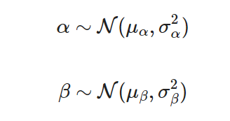
Keeping with simplicity in this example, I will assume that the intercept and slope each come from a normal distribution with a mean and variance such that:
When it comes time to make inferences or predictions using our model, we can create a large number of predictions by sampling different parameter values from these distributions. Consequently, we will end up with a distribution of uncertain predictions.
NOTE: The MCMC sampler used by PyMC is written in C and will be SIGNIFICANTLY faster if you provide have access to GCC compiler and specify the it’s directory using the the following:
import pymc as pm

import os
os.environ["THEANO_FLAGS"] = "gcc__cxxflags=-C:\mingw-w64\mingw64\bin"
You will get a warning if you don’t have this properly set up.
Now, onto the demo!
I start by retrieving our X and Y data from the CAMELS dataset we created above:
# Pull out X and Y of interest
x_ftr= 'area_gages2'
y_ftr = 'q_mean_cms'
xs = camels_basins[x_ftr]
ys = camels_basins[y_ftr]

# Take log-transform
xs = np.log(xs)
ys = np.log(ys)
At a glance, we see there is a reasonable linear relationship when working in the log space:
Two of the key features when building a model are:
The random variable distribution constructions
The deterministic model formulation
There are lots of different distributions available, and each one simply takes a name and set of parameter values as inputs. For example, the normal distribution defining our intercept parameter is:
The value of the parameter priors that you specify when construction the model may have a big impact depending on the complexity of your model. For simple models you may get away with having uninformative priors (e.g., setting mu=0), however if you have some initial guesses then that can help with getting reliable convergence.
In this case, I used a simple least squares estimate of the linear regression as the parameter priors:
Once we have our random variables defined, then we will need to formulate the deterministic element of our model prediction. This is the functional relationship between the input, parameters, and output. For our linear regression model, this is simply:
y_mu = alpha + beta * xs
In the case of our Bayesian regression, this can be thought of as the mean of the regression outputs. The final estimates are going to be distributed around the y_mu with the uncertainty resulting from the combinations of our different random variables.
Putting it all together now:
### PyMC linear model
with pm.Model() as model:

    # Priors
    alpha = pm.Normal('alpha', mu=intercept_prior, sigma=10)
    beta = pm.Normal('beta', mu=slope_prior, sigma=10)
    sigma = pm.HalfNormal('sigma', sigma=1)

    # mean/expected value of the model
    mu = alpha + beta * xs

    # likelihood
    y = pm.Normal('y', mu=mu, sigma=sigma, observed=ys)

    # sample from the posterior
    trace = pm.sample(2000, cores=6)
With our model constructed, we can use the pm.sample() function to begin the MCMC sampling process and estimate the posterior distribution of model parameters. Note that this process can be very computationally intensive for complex models! (Definitely make sure you have the GCC set up correctly if you plan on needing to sample complex models.)
Using the sampled parameter values, we can create posterior estimates of the predictions (log mean flow) using the posterior parameter distributions:
Let’s go ahead and plot the range of the posterior distribution, to visualize the uncertainty in the model estimates:
### Plot the posterior predictive interval
fig, ax = plt.subplots(ncols=2, figsize=(8,4))

# log space
az.plot_hdi(xs, ppc['posterior_predictive']['y'],
            color='cornflowerblue', ax=ax[0], hdi_prob=0.9)
ax[0].scatter(xs, ys, alpha=0.6, s=20, color='k')
ax[0].set_xlabel('Log ' + x_ftr)
ax[0].set_ylabel('Log Mean Flow (m3/s)')

# original dim space
az.plot_hdi(np.exp(xs), np.exp(ppc['posterior_predictive']['y']),
            color='cornflowerblue', ax=ax[1], hdi_prob=0.9)
ax[1].scatter(np.exp(xs), np.exp(ys), alpha=0.6, s=20, color='k')
ax[1].set_xlabel(x_ftr)
ax[1].set_ylabel('Mean Flow (m3/s)')
plt.suptitle('90% Posterior Prediction Interval', fontsize=14)
plt.show()
And there we have it! The figure on the left shows the data and posterior prediction range in log-space, while the figure on the right is in non-log space.
As mentioned earlier, it’s not the best model (wayyy to much uncertainty in the large-basin mean flow estimates), but at least we have the benefit of knowing the uncertainty distribution since we took the Bayesian approach!
That’s all for now; this post was really meant to bring PyMC to your attention. Maybe you have a use case or will be more likely to consider Bayesian approaches in the future.
If you have other Bayesian/probabilistic programming tools that you like, please do comment below. PyMC is one (good) option, but I’m sure other people have their own favorites for different reasons.
Addor, N., Newman, A. J., Mizukami, N. and Clark, M. P. The CAMELS data set: catchment attributes and meteorology for large-sample studies, Hydrol. Earth Syst. Sci., 21, 5293–5313, doi:10.5194/hess-21-5293-2017, 2017.
The line_profiler can be used to see the amount of time taken to execute each line in a function of your code. I think this is an important tool that can be used to reduce the runtime of a code. Simple command “pip install line_profiler” shall install the package or “conda install line_profiler” to install into an existing conda environment.
I shall present the usage of this line_profiler tool for a randomly generated data to calculate supply to demand ratio for releases from a reservoir. Demand or target supply is defined for day of the water year. The following code first defines the calculation for day of water year, generates random data for demand and supply, and two functions are defined for different methods of calculation of ratio of supply to demand. Include the line @profile before the function definition line to get the profile of execution of each line in the function.
import pandas as pd import numpy as np from line_profiler import profile
#function to caluclate day of water year def get_dowy(date): water_year_start = pd.Timestamp(year=date.year, month=10, day=1) if date < water_year_start: water_year_start = pd.Timestamp(year=date.year - 1, month=10, day=1) return (date - water_year_start).days + 1
# Generate random data for demand for each day of water year np.random.seed(0) data = { 'Median_Demand': np.random.randint(0, 1000, 367), }
# Create dataframe df_demand = pd.DataFrame(data)
## Generate random data for supply from years 2001 to 2010 and also define corresponding day of water year date_range = pd.date_range(start='2001-10-01', end='2091-09-30', freq='D') data = { 'dowy': [get_dowy(date) for date in date_range], 'Supply': np.random.uniform(0, 2500, len(date_range)) } # Create dataframe df_supply = pd.DataFrame(data, index=date_range)
@profile #define before the function for profiling def calc_supply_demand_1(df,df_median): ratio = pd.DataFrame() medians_dict = df_demand['Median_Demand'].to_dict() demand = df_supply['dowy'].map(medians_dict) supply = df_supply['Supply'] ratio = supply.resample('AS-OCT').sum() / demand.resample('AS-OCT').sum() return ratio
@profile def calc_supply_demand_2(df,df_median): ratio = pd.DataFrame() medians_dict = df_demand['Median_Demand'].to_dict() demand = pd.Series([df_demand['Median_Demand'][i] for i in df.dowy], index=df.index) supply = df_supply['Supply'] ratio = supply.resample('AS-OCT').sum() / demand.resample('AS-OCT').sum() return ratio
Running just the code wouldn’t output anything related to line_profiler. To enable profiling, run the script as follows (this sets the environment variable LINE_PROFILE=1)
LINE_PROFILE=1 python Blog_Post.py
The above line generates three output files as profile_output.txt, profile_output_.txt, and profile_output.lprof and stdout is as follows:
Timer unit: 1e-09 s

  0.04 seconds - /directory/Blog_Post.py:30 - calc_supply_demand_1
  2.43 seconds - /directory/Blog_Post.py:39 - calc_supply_demand_2
Wrote profile results to profile_output.txt
Wrote profile results to profile_output_2024-03-29T192919.txt
Wrote profile results to profile_output.lprof
To view details run:
python -m line_profiler -rtmz profile_output.lprof
On executing the line “python -m line_profiler -rtmz profile_output.lprof”, the following is printed.
Timer unit: 1e-06 s
Total time: 0.0393394 s File: /directory/Blog_Post.py Function: calc_supply_demand_1 at line 30
Line # Hits Time Per Hit % Time Line Contents ============================================================== 30 @profile 31 def calc_supply_demand_1(df,df_median): 32 1 2716.4 2716.4 6.9 ratio = pd.DataFrame() 33 1 1365.2 1365.2 3.5 medians_dict = df_demand['Median_Demand'].to_dict() 34 1 3795.6 3795.6 9.6 demand = df_supply['dowy'].map(medians_dict) 35 1 209.7 209.7 0.5 supply = df_supply['Supply'] 36 1 31252.0 31252.0 79.4 ratio = supply.resample('AS-OCT').sum() / demand.resample('AS-OCT').sum() 37 1 0.5 0.5 0.0 return ratio
Total time: 2.43446 s File: /directory/Blog_Post.py Function: calc_supply_demand_2 at line 39
Line # Hits Time Per Hit % Time Line Contents ============================================================== 39 @profile 40 def calc_supply_demand_2(df,df_median): 41 1 1365.1 1365.1 0.1 ratio = pd.DataFrame() 42 1 697.5 697.5 0.0 medians_dict = df_demand['Median_Demand'].to_dict() 43 1 2411800.5 2e+06 99.1 demand = pd.Series([df_demand['Median_Demand'][i] for i in df.dowy], index=df.index) 44 1 53.9 53.9 0.0 supply = df_supply['Supply'] 45 1 20547.0 20547.0 0.8 ratio = supply.resample('AS-OCT').sum() / demand.resample('AS-OCT').sum() 46 1 0.6 0.6 0.0 return ratio
The result shows line number, number of hits (number of times the line is executed; hits increase when executed in a for loop), total time, time per hit, percentage of time and the line contents. The above result implies that for the first function, 79.4% of time was used to execute ratio, whereas for the second function 99.1% is used in execution of demand. ratio1 and ratio2 are the two exact same outputs where demand is defined in different ways in both the functions. We also see that time taken to execute calc_supply_demand_1 function is 0.04 seconds and calc_supply_demand_2 is 2.43 seconds. Using this I could reduce the runtime by 61 times (2.43/0.04) identifying that demand calculation takes 99.1% of time in calc_supply_demand_2 function using line_profiler. Another method is using cprofile (details are in this blog post). cprofile gives more detailed information.
In Parallel Programming Part 1, I introduced a number of basic OpenMP directives and constructs, as well as provided a quick guide to high-performance computing (HPC) terminology. In Part 2 (aka this post), we will apply some of the constructs previously learned to execute a few OpenMP examples. We will also view an example of incorrect use of OpenMP constructs and its implications.
TheCube Cluster Setup
Before we begin, there are a couple of steps to ensure that we will be able to run C++ code on the Cube. First, check the default version of the C++ compiler. This compiler essentially transforms your code into an executable file that can be easily understood and implemented by the Cube. You can do this by entering
g++ --version
into your command line. You should see that the Cube has G++ version 8.3.0 installed, as shown below.
Now, create two files:
openmp-demo-print.cpp this is the file where we will perform a print demo to show how tasks are distributed between threads
openmp-demo-access.cpp this file will demonstrate the importance of synchronization and the implications if proper synchronization is not implemented
Example 1: Hello from Threads
Open the openmp-demo-print.cpp file, and copy and paste the following code into it:
#include <iostream>
#include <omp.h>
#include <stdio.h>

int main() {

    int num_threads = omp_get_max_threads(); // get max number of threads available on the Cube
    omp_set_num_threads(num_threads);

    printf("The CUBE has %d threads.\n", num_threads);


    #pragma omp parallel
    {
        int thread_id = omp_get_thread_num();
        printf("Hello from thread num %d\n", thread_id);
    }

    printf("Thread numbers written to file successfully. \n");

    return 0;
}
Here is what the code is doing:
Lines 1 to 3 are the libraries that need to be included in this script to enable the use of OpenMP constructs and printing to the command line.
In main() on Lines 7 and 8, we first get the maximum number of threads that the Cube has available on one node and assign it to the num_threads variable. We then set the number of threads we want to use.
Next, we declare a parallel section using #pragma omp parallel beginning on Line 13. In this section, we are assigning the printf() function to each of the num_threads threads that we have set on Line 8. Here, each thread is now executing the printf() function independently of each other. Note that the threads are under no obligation to you to execute their tasks in ascending order.
Finally, we end the call to main() by returning 0
Be sure to first save this file. Once you have done this, enter the following into your command line:
This tells the system to compile openmp-demo-print.cpp and create an executable object using the same file name. Next, in the command line, enter:
./openmp-demo-print
You should see the following (or some version of it) appear in your command line:
Notice that the threads are all being printed out of order. This demonstrates that each thread takes a different amount of time to complete its task. If you re-run the following script, you will find that the order of threads that are printed out would have changed, showing that there is a degree of uncertainty associated with the amount of time they each require. This has implications for the order in which threads read, write, and access data, which will be demonstrated in the next example.
Example 2: Who’s (seg)Fault Is It?
In this example, we will first execute a script that stores each thread number ID into an array. Each thread then accesses its ID and prints it out into a text file called access-demo.txt. See the implementation below:
#include <iostream>
#include <omp.h>
#include <vector>

using namespace std;

void parallel_access_demo() {
    vector<int> data;
    int num_threads = omp_get_max_threads();

    // Parallel region for appending elements to the vector
    #pragma omp parallel for
    for (int i = 0; i < num_threads; ++i) {
        // Append the thread ID to the vector
        data.push_back(omp_get_thread_num()); // Potential race condition here
    }
}

int main() {
    // Execute parallel access demo
    parallel_access_demo();
    printf("Code ran successfully. \n");

    return 0;
}
As per the usual, here’s what’s going down:
After including the necessary libraries, we use include namespace std on Line 5 so that we can more easily print text without having to used std:: every time we attempt to write a statement to the output file
Starting on Line 7, we write a simple parallel_access_demo() function that does the following:
Initialize a vector of integers very creatively called data
Get the maximum number of threads available per node on the Cube
Declare a parallel for region where we iterate through all threads and push_back the thread ID number into the data vector
Finally, we execute this function in main() beginning Line 19.
If you execute this using a similar process shown in Example 1, you should see the following output in your command line:
Congratulations – you just encountered your first segmentation fault! Not to worry – this is by design. Take a few minutes to review the code above to identify why this might be the case.
Notice Line 15. Where, each thread is attempting to insert a new integer into the data vector. Since push_back() is being called in a parallel region, this means that multiple threads are attempting to modify data simultaneously. This will result in a race condition, where the size of data is changing unpredictably. There is a pretty simple fix to this, where we add a #pragma omp criticalbefore Line 15.
As mentioned in Part 1, #pragma omp critical ensures that each thread executes its task one at a time, and not all at once. It essentially serializes a portion of the parallel for loop and prevents race conditions by ensuring that the size of data changes in a predictable and controlled manner. An alternative would be to declare #pragma omp single in place of #pragma omp parallel foron Line 12. This essentially delegates the following for-loop to a single thread, forcing the loop to be completed in serial. Both of these options will result in the blissful outcome of
Summary
In this post, I introduced two examples to demonstrate the use of OpenMP constructs. In Example 1, I demonstrated a parallel printing task to show that threads do not all complete their tasks at the same time. Example 2 showed how the lack of synchronization can lead to segmentation faults due to race conditions, and two methods to remedy this. In Part 3, I will introduce GPU programming using the Python PyTorch library and Google Colaboratory cloud infrastructure. Until then, happy coding!
In this post, I will describe the motivation for and implementation of a nonstationary stochastic watershed modeling (SWM) approach that we developed in the Steinschneider group during the course of my PhD. This work is in final revision and should be published in the next month or so. This post will attempt to distill key components of the model and their motivation, saving the full methodological development for those who’d like to read the forthcoming paper.
SWMs vs SSM/SSG
Before diving into the construction of the model, some preliminaries are necessary. First, what are SWMs, what do they do, and why use them? SWMs are a framework that combine deterministic, process-based watershed models (think HYMOD, SAC-SMA, etc.; we’ll refer to these as DWMs from here forward) with a stochastic model that capture their uncertainty. The stochastic part of this framework can be used to generate ensembles of SWM simulations that both represent the hydrologic uncertainty and are less biased estimators of the streamflow observations (Vogel, 2017).
Figure 1: SWM conceptual diagram
SWMs were developed to address challenges to earlier stochastic streamflow modeling/generation techniques (SSM/SSG; see for instance Trevor’s post on the Thomas-Fiering SSG; Julie’s post and Lillian’s post on other SSG techniques), the most important of which (arguably) being the question of how to formulate them under non-stationarity. Since SSMs are statistical models fitted directly to historical data, any attempt to implement them in a non-stationary setting requires strong assumptions about what the streamflow response might look like under an alternate forcing scenario. This is not to say that such an approach is not useful or valid for exploratory analyses (for instance Rohini’s post on synthetic streamflow generation to explore extreme droughts). SWMs attempt to address this issue of non-stationarity by using DWMs in their stochastic formulation, which lend some ‘physics-based’ cred to their response under alternate meteorological forcings.
Construction of an SWM
Over the years, there have been many SWM or SWM-esque approaches devised, ranging from simple autoregressive models to complex Bayesian approaches. In this work, we focus on a relatively straightforward SWM approach that models the hydrologic predictive uncertainty directly and simply adds random samples of it to the DWM simulations. The assumption here being that predictive uncertainty is an integrator of all traditional component modeling uncertainties (input, parameter, model/structural), so adding it back in can inject all these uncertainties into the SWM simulations at once (Shabestanipour et al., 2023).
Figure 2: Uncertainty components
By this straightforward approach, the fitting and parameter estimation of the DWM is accomplished first (and separately) via ‘standard’ fitting procedures; for instance, parameter optimization to minimize Nash-Sutcliffe Efficiency (NSE). Subsequently, we develop our stochastic part of the model on the predictive uncertainty that remains, which in this case, is defined simply by subtracting the target observations from the DWM predictions. This distribution of differenced errors is the ‘predictive uncertainty distribution’ or ‘predictive errors’ that form the target of our stochastic model.
Challenges in modeling predictive uncertainty
Easy, right? Not so fast. There is a rather dense and somewhat unpalatable literature (except for the masochists out there) on the subject of hydrologic uncertainty that details the challenges in modeling these sorts of errors. Suffice it to say that they aren’t well behaved. Any model we devise for these errors must be able to manage these bad behaviors.
So, what if we decide that we want to try to use this SWM thing for planning under future climates? Certainly the DWM part can hack it. We all know that lumped, conceptual DWMs are top-notch predictors of natural streamflow… At the least, they can produce physically plausible simulations under alternate forcings (we think). What of the hydrologic predictive uncertainty then? Is it fair or sensible to presume that some model we constructed to emulate historical uncertainty is appropriate for future hydrologic scenarios with drastically different forcings? My line of rhetorical questioning should clue you in on my feelings on the subject. YES!, of course. ‘Stationarity is immortal!’ (Montanari & Koutsoyiannis, 2014).
Towards a hybrid, state-variable dependent SWM
No, actually, there are a number of good reasons why this statement might not hold for hydrologic predictive uncertainty under non-stationarity. You can read the paper for the laundry list. In short, hydrologic predictive uncertainty of a DWM is largely a reflection of its structural misrepresentation of the true process. Thus, the historical predictive uncertainty that we fit our model to is a reflection of that structural uncertainty propagated through historical model states under historical, ‘stationary’ forcings. If we fundamentally alter those forcings, we should expect to see model states that do not exist under historical conditions. The predictive errors that result from these fundamentally new model states are thus likely to not fall neatly into the box carved out by the historical scenarios.
Figure 3: Structural uncertainty
To bring this back to the proposition for a nonstationary SWM approach. The intrinsic link between model structure and its predictive uncertainty raises an interesting prospect. Could there be a way to leverage a DWM’s structure to understand its predictive uncertainty? Well, I hope so, because that’s the premise of this work! What I’ll describe in the ensuing sections is the implementation of a hybrid, state-variable dependent SWM approach. ‘Hybrid’ because it couples both machine learning (ML) and traditional statistical techniques. ‘State-variable dependent’ because it uses the timeseries of model states (described later) as the means to infer the hydrologic predictive uncertainty. I’ll refer to this as the ‘hybrid SWM’ for brevity.
Implementation of the hybrid SWM
So, with backstory in hand, let’s talk details. The remainder of this post will describe the implementation of this hybrid SWM. This high-level discussion of the approach supports a practical training exercise I put together for the Steinschneider group at the following public GitHub repo: https://github.com/zpb4/hybrid-SWM_training. This training also introduces a standard implementation of a GRRIEN repository (see Rohini’s post). Details of implementing the code are contained in the ‘README.md’ and ‘training_exercise.md’ files in the repository. My intent in this post is to describe the model implementation at a conceptual level.
Model-as-truth experimental design
First, in order to address the problem of non-stationary hydrologic predictive uncertainty, we need an experimental design that can produce it. There is a very real challenge here of not having observational data from significantly altered climates to compare our hydrologic model against. We address this problem by using a ‘model-as-truth’ experimental design, where we fit one hydrologic model (‘truth’ model) to observations, and a second hydrologic model (‘process’ model) to the first truth model. The truth model becomes a proxy for the true, target flow of the SWM modeling procedure, while the process model serves as our proposed model, or hypothesis, about that true process. Under this design, we can force both models with any plausible forcing scenario to try to understand how the predictive uncertainty between ‘truth’ and ‘process’ models might change.
Figure 4: Conceptual diagram of ‘model-as-truth’ experimental design
For the actual work, we consider a very simple non-stationary scenario where we implement a 4oC temperature shift to the temperature forcing data, which we refer to as the ‘Test+4C’ scenario. We choose this simple approach to confine non-stationarity to a high-confidence result of anthropogenic climate change, namely, thermodynamic warming. We compare this Test+4C scenario to a ‘Test’ scenario, which is the same out-of-sample temporal period (WY2005-2018) of meteorological inputs under historical values. SAC-SMA and HYMOD are the truth model and process model for this experiment, respectively. Other models could have been chosen. We chose these because they are conceptually similar and commonly used.
Figure 5: Errors between truth and process models in 5 wettest years of Test/Test+4C scenarios.
Hybrid SWM construction
The core feature of the hybrid SWM is a model for the predictive errors (truth model – process model) that uses the hydrologic model state-variables as predictors. We implement this model in two steps that have differing objectives, but use the same state-variable predictor information. An implicit assumption in using state-variable dependencies in both steps is that these dependencies can exist in both stages. In other words, we do not expect the error-correction step to produce independent and identically distributed residuals. We call the first step an ‘error-correction model’ and the second step a ‘dynamic residual model’. Since we use HYMOD as our process model, we use its state-variables (Table 1) as the predictors for these two steps.
Table 1: HYMOD state variables
Short Name
Long Name
Description
sim
Simulation
HYMOD predicted streamflow in mm
runoff
Runoff
Upper reservoir flow of HYMOD in mm
baseflow
Baseflow
Lower reservoir flow of HYMOD in mm
precip
Precipitation
Basin averaged precipitation in mm
tavg
Average temperature
Basin averaged temperature in oC
et
Evapotranspiration
Modeled evapotranspiration (Hamon approach) in mm
upr_sm
Upper soil moisture
Basin averaged soil moisture content (mm) in upper reservoir
lwr_sm
Lower soil moisture
Basin averaged soil moisture (mm) in lower reservoir
swe
Snow water equivalent
Basin averaged snow water equivalent simulated by degree day snow module (mm)
Hybrid SWM: Error correction
The error-correction model is simply a predictive model between the hydrologic model (HYMOD) state-variables and the raw predictive errors. The error-correction model also uses lag-1 to 3 errors as covariates to account for autocorrelation. The objective of this step is to infer state-dependent biases in the errors, which are the result of the predictive errors subsuming the structural deficiencies of the hydrologic model. This ‘deterministic’ behavior in the predictive errors can also be conceived as the ‘predictive errors doing what the model should be doing’ (Vogel, 2017). Once this error-correction model is fit to its training data, it can be implemented against any new timeseries of state-variables to predict and debias the errors. We use a Random Forest (RF) algorithm for this step because they are robust to overfitting, even with limited training data. This is certainly the case here, as we consider only individual basins and a ~15 year training period (WY1989-2004). Moreover, we partition the training period into a calibration and validation subset and fit the RF error-correction model only to the calibration data (WY1989-1998), reducing available RF algorithm training data to 9 years.
Hybrid SWM: Dynamic residual model
The dynamic residual model (DRM) is fit to the residuals of the error correction result in the validation subset. We predict the hydrologic model errors for the validation subset from the fitted RF model and subtract them from the empirical errors to yield the residual timeseries. By fitting the DRM to this separate validation subset (which the RF error-correction model has not seen), we ensure that the residuals adequately represent the out-of-sample uncertainty of the error-correction model.
A full mathematical treatment of the DRM is outside the scope of this post. In high-level terms, the DRM is built around a flexible distributional form particularly suited to hydrologic errors, called the skew exponential power (SEP) distribution. This distribution has 4 parameters (mean: mu, stdev: sigma, kurtosis: beta, skew: xi) and we assume a mean of zero (due to error-correction debiasing), while setting the other 3 parameters as time-varying predictands of the DRM model (i.e. sigmat, betat, xit). We also include a lag-1 autocorrelation term (phit) to account for any leftover autocorrelation from the error-correction procedure. We formulate a linear model for each of these parameters with the state-variables as predictors. These linear models are embedded in a log-likelihood function that is maximized (i.e. MLE) against the residuals to yield the optimal set of coefficients for each of the linear models.
With a fitted model, the generation of a new residual at each timestep t is therefore a random draw from the SEP with parameters (mu=0, sigmat, betat, xit) modified by the residual at t-1 (epsilont-1) via the lag-1 coefficient (phit).
Figure 6: Conceptual diagram of hybrid SWM construction.
Hybrid SWM: Simulation
The DRM is the core uncertainty modeling component of the hybrid SWM. Given a timeseries of state-variables from the hydrologic model for any scenario, the DRM simulation is implemented first, as described in the previous section. Subsequently, the error-correction model is implemented in ‘predict’ mode with the timeseries of random residuals from the DRM step. Because the error-correction model includes lag-1:3 terms, it must be implemented sequentially using errors generated at the previous 3 timesteps. The conclusion of these two simulation steps yields a timeseries of randomly generated, state-variable dependent errors that can be added to the hydrologic model simulation to produce a single SWM simulations. Repeating this procedure many times will produce an ensemble of SWM simulations.
Final thoughts
Hopefully this discussion of the hybrid SWM approach has given you some appreciation for the nuanced differences between SWMs and SSM/SSGs, the challenges in constructing an adequate uncertainty model for an SWM, and the novel approach developed here in utilizing state-variable information to infer properties of the predictive uncertainty. The hybrid SWM approach shows a lot of potential for extracting key attributes of the predictive errors, even under unprecedented forcing scenarios. It decouples the task of inferring predictive uncertainty from features of the data like temporal seasonality (e.g. day of year) that may be poor predictors under climate change. When linked with stochastic weather generation (see Rohini’s post and Nasser’s post), SWMs can be part of a powerful bottom-up framework to understand the implications of climate change on water resources systems. Keep an eye out for the forthcoming paper and check out the training noted above on implementation of the model.
References:
Brodeur, Z., Wi, S., Shabestanipour, G., Lamontagne, J. R., & Steinschneider, S. A hybrid, non-stationary Stochastic Watershed Model (SWM) for uncertain hydrologic simulations under climate change. Water Resources Research, in review.
Montanari, A., & Koutsoyiannis, D. (2014). Modeling and mitigating natural hazards: Stationarity is immortal! Water Resources Research, 50, 9748–9756. https://doi.org/10.1002/ 2014WR016092
Shabestanipour, G., Brodeur, Z., Farmer, W. H., Steinschneider, S., Vogel, R. M., & Lamontagne, J. R. (2023). Stochastic Watershed Model Ensembles for Long-Range Planning : Verification and Validation. Water Resources Research, 59. https://doi.org/10.1029/2022WR032201
In my recent Applied High Performance Computing (HPC) lectures, I have been learning to better utilize OpenMP constructs and functions . If these terms mean little to nothing to you, welcome to the boat – it’ll be a collaborative learning experience. For full disclosure, this blog post assumes some basic knowledge of parallel programming and its related terminology. But just in case, here is a quick glossary:
Node: One computing unit within a supercomputing cluster. Can be thought of as on CPU unit on a traditional desktop/laptop.
Core: The physical processing unit within the CPU that enables computations to be executed. For example, an 11th-Gen Intel i5 CPU has four cores.
Processors/threads: Simple, lightweight “tasks” that can be executed within a core. Using the same example as above, this Intel i5 CPU has eight threads, indicating that each of its cores can run two threads simultaneously.
Shared memoryarchitecture: This means that all cores share the same memory within a CPU, and are controlled by the same operating system. This architecture is commonly found in your run-of-the-mill laptops and desktops.
Distributed memory architecture: Multiple cores run their processes independently of each other. They communicate and exchange information via a network. This architecture is more commonly found in supercomputer clusters.
Serial execution: Tasks and computations are completed one at a time. Typically the safest and most error-resistant form of executing tasks, but is the least efficient.
Parallel execution: Tasks and computations are completed simultaneously. Faster and more efficient than serial execution, but runs the risk of errors where tasks are completed out of order.
Synchronization: The coordination of multiple tasks or computations to ensure that all processes aligns with each other and abide by a certain order of execution. Synchronization takes up more time than computation. AN overly-cautious code execution with too many synchronization points can result in unnecessary slowdown. However, avoiding it altogether can result in erroneous output due to out-of-order computations.
Race condition: A race condition occurs when two threads attempt to access the same location on the shared memory at the same time. This is a common problem when attempting parallelized tasks on shared memory architectures.
Load balance: The distribution of work (tasks, computations, etc) across multiple threads. OpenMP implicitly assumes equal load balance across all its threads within a parallel region – an assumption that may not always hold true.
This is intended to be a two-part post where I will first elaborate on the OpenMP API and how to use basic OpenMP clauses to facilitate parallelization and code speedup. In the second post, I will provide a simple example where I will use OpenMP to delineate my code into serial and parallel regions, force serialization, and synchronize memory accesses and write to prevent errors resulting from writing to the same memory location simultaneously.
What is OpenMP?
OpenMP stands for “Open Specification for Multi-Processing”. It is an application programming interface (API) that enables C/C++ or Fortran code to “talk” (or interface) with multiple threads within and across multiple computing nodes on shared memory architectures, therefore allowing parallelism. It should not be confused with MPI (Message Passing Interface), which is used to develop parallel programs on distributed memory systems (for a detailed comparison, please refer to this set of Princeton University slides here). This means that unlike a standalone coding language like C/C++. Python, R, etc., it depends only on a fixed set of simple implementations using lightweight syntax (#pragma omp [clause 1] [clause 2]) . To begin using OpenMP, you should first understand what it can and cannot do.
Things you can do with OpenMP
Explicit delineation of serial and parallel regions
One of the first tasks that OpenMP excels at is the explicit delineation of your code into serial and parallel regions. For example:
In the code block above, we are delineating an entire parallel region where the task performed by the do_a_parallel_task() function is performed independently by each thread on a single node. The number of tasks that can be completed at any one time depends on the number of threads that are available on a single node.
Hide stack management
In addition, using OpenMP allows you toautomate memory allocation, or “hide stack management”. Most machines are able to read, write, and (de)allocate data to optimize performance, but often some help from the user is required to avoid errors caused by multiple memory access or writes . OpenMP allows the user to automate stack management without explicitly specifying memory reads or writes in certain cache locations via straightforward clauses such as collapse() (we will delve into the details of such clauses in later sections of this blog post).
Allow synchronization
OpenMP also provides synchronization constructs to enforce serial operations or wait times within parallel regionsto avoid conflicting or simultaneous read or write operations where doing so might result in erroneous memory access or segmentation faults. For example, a sequential task (such as a memory write to update the value in a specific location) that is not carefully performed in parallel could result in output errors or unexpected memory accessing behavior. Synchronization ensures that multiple threads have to wait until the last operation on the last thread is completed, or only one thread is allowed to perform an operation at a time. It also protects access to shared data to prevent multiple reads (false sharing). All this can be achieved via the critical, barrier, or single OpenMP clauses.
Creating a specific number of threads
Unless explicitly stated, the system will automatically select the number of threads (or processors) to use for a specific computing task. Note that while you can request for a certain number of threads in your environment using export OMP_NUM_THREADS, the number of threads assigned to a specific task is set by the system unless otherwise specified. OpenMP allows you to control the number of threads you want to use in a specific task in one of two ways: (a) using omp_set_num_threads() and using (b) #pragma omp parallel [insert num threadshere]. The former allows you to enforce an upper limit of the number of threads to be freely assigned to tasks throughout the code, while the latter allows you to specify a set number of threads to perform an operation(s) within a parallel region.
In the next section, we will list some commonly-used and helpful OpenMP constructs and provide examples of their use cases.
OpenMP constructs and their use cases
OMP_NUM_THREADS This is an environment variable that can be set either in the section of your code where you defined your global variables, or in the SLURM submission script you are using to execute your parallel code.
omp_get_num_threads() This function returns the number of threads currently executing the parallel region from which it is called. Use this to gauge how many active threads are being used within a parallel region
omp_set_num_threads() This function specifies the number of threads to use for any following parallel regions. It overrides the OMP_NUM_THREADS environment variable. Be careful to not exceed the maximum number of threads available across all your available cores. You will encounter an error otherwise.
omp_get_max_threads() To avoid potential errors from allocating too many threads, you can use omp_set_num_threads() with omp_get_max_threads(). This returns the maximum number of threads that can be used to form a new “team” of threads in a parallel region.
#pragma omp parallel This directive instructs your compiler to create a parallel region within which it instantiates a set (team) of threads to complete the computations within it. Without any further specifications, the parallelization of the code within this block will be automatically determined by the compiler.
#pragma omp for Use this directive to instruct the compiler to parallelize for-loop iterations within the team of threads that it has instantiated. This directive is often used in combination with #pragma omp parallel to form the #pragma omp parallel for construct which both creates a parallel region and distributes tasks across all threads.
To demonstrate:
#include <stdio.h>
#include <omp.h>
void some_function() {
	#pragma omp parallel {
        #pragma omp for
		for (int i = 0; i < some_num; i++) {
             perform_task_here();
        }
	}
}
is equivalent to
#include <stdio.h>
#include <omp.h>
void some_function() {
	#pragma omp parallel for {
    for (int i = 0; i < some_num; i++) {
          perform_task_here();
     }
}
#pragma omp barrier This directive marks the start of a synchronization point. A synchronization point can be thought of as a “gate” at which all threads must wait until all remaining threads have completed their individual computations. The threads in the parallel region beyond omp barrier will not be executed until all threads before is have completed all explicit tasks.
#pragma omp single This is the first of three synchronization directives we will explore in this blog post. This directive identifies a section of code, typically contained within “{ }”, that can only be run with one thread. This directive enforces serial execution, which can improve accuracy but decrease speed. The omp single directive imposes an implicit barrier where all threads after #pragma omp single will not be executed until the single thread running its tasks is done. This barrier can be removed by forming the #pragma omp single nowait construct.
#pragma omp master This directive is similar to that of the #pragma omp single directive, but chooses only the master thread to run the task (the thread responsible creating, managing and discarding all other threads). Unlike #pragma omp single, it does not have an implicit barrier, resulting in faster implementations. Both #pragma omp single and #pragma omp master will result in running only a section of code once, and it useful for controlling sections in code that require printing statements or indicating signals.
#pragma omp critical A section of code immediate following this directive can only be executed by one thread at a time. It should not be confused with #pragma omp single. The former requires that the code be executed by one thread at a time, and will be executed as many times as has been set byomp_set_num_threads(). The latter will ensure that its corresponding section of code be executed only once. Use this directive to prevent race conditions and enforce serial execution where one-at-a-time computations are required.
Things you cannot (and shouldn’t) do with OpenMP
As all good things come to an end, all HPC APIs must also have limitations. In this case, here is a quick rundown in the case of OpenMP:
OpenMP is limited to function on shared memory machines and should not be run on distributed memory architectures.
It also implicitly assumes equal load balance. Incorrectly making this assumption can lead to synchronization delays due to some threads taking significantly longer to complete their tasks compared to others immediately prior to a synchronization directive.
OpenMP may have lower parallel efficiency due to it functioning on shared memory architectures, eventually being limited by Amdahl’s law.
It relies heavily on parallelizable for-loops instead of atomic operations.
Summary
In this post, we introduced OpenMP and a few of its key constructs. We also walked through brief examples of their use cases, as well as limitations of the use of OpenMP. In our next blog post, we will provide a tutorial on how to write, compile, and run a parallel for-loop on Cornell’s Cube Cluster. Until then, feel free to take a tour through the Cornell Virtual Workshop course on OpenMP to get a head start!
This is a guest post by David Lafferty from the University of Illinois Urbana-Champaign. David is a fifth-year PhD student in the Department of Climate, Meteorology & Atmospheric Sciences working with Dr. Ryan Sriver. David’s research contributes to advances in climate change risk assessment. Dr. Casey Burleyson, a research scientist at the Pacific Northwest National Laboratory, also contributed text about the MSD-LIVE platform.
Visualization plays a crucial role in the scientific process. From an initial exploratory data analysis to the careful presentation of hard-earned results, data visualization is a powerful tool to generate hypotheses and insights, communicate findings to both scientists and stakeholders, and aid decision-making. Interactive data visualization can enhance each of these use cases and is particularly useful for facilitating collaborations and deepening user engagement. Effective data visualization has been a recurring theme of the Water Programming blog, with several past posts directly addressing the topic, including some that highlight various tools for interactive visualization [1, 2].
In this post, I’d like to highlight Panel, a data exploration and web app framework in Python. I’ll also showcase how we used Panel to construct an interactive dashboard to accompany a recent paper, allowing readers to explore our results in more detail.
An overview of the HoloViz ecosystem, taken from the hvPlot website. Panel provides a high-level interface that allows users to build linked apps across all of these visualization libraries.
Panel is an open-source Python library that allows developers to create interactive web apps and dashboards in Python. It is part of the HoloViz ecosystem, which includes other visualization packages like HoloViews and GeoViews. Panel provides a high-level API for creating rich, interactive visualizations and user interfaces directly from Python code. The library includes an impressive number of features, such as different types of panes for displaying and arranging plots, media, text, or other external objects; a wide range of widgets; and flexible, customizable dashboard layouts. Panel itself does not provide visualization tools but instead relies on (and is designed to work well with) other popular plotting libraries such as Bokeh, Datashader, Folium, Plotly, and Matplotlib. Panel provides several deployment options for your polished apps and dashboards, but also works well within development environments such as Jupyter Notebooks, VS Code, PyCharm, or Spyder.
A simple Panel dashboard
To get a sense of Panel’s capabilities, let’s build a simple dashboard that analyzes global temperature anomalies from different observational datasets. Global mean temperature rise above pre-industrial levels is one of most widely-used indicators of climate change, and 2023 was a record year in this respect – all major monitoring agencies recorded 2023 as the warmest year on record [3] and the exceptional warmth of 2023 fell outside the prediction intervals of many forecasting groups [4].
To visualize this temperature change, we’re going to look at four observational datasets: Berkeley Earth, HadCRUT5, NOAA, and GISTEMPv4. First, we need to import the required Python libraries:
!pip install hvplot

from functools import reduce
import pandas as pd
import hvplot.pandas

import panel as pn
pn.extension(comms='colab')
This notebook is available on Google Colab, which is why I’ve set comms=‘colab' in the Panel configuration settings. Next, we download and merge all observational datasets:
As you can see, each of these datasets measures the global mean temperature anomaly relative to a fixed baseline, and the baselines are not constant across datasets. Climate scientists often define 1850-1900 as the canonical pre-industrial baseline, but choosing this period is a non-trivial exercise [5] and can impact the uncertainty around our estimates of climate change. Let’s explore this phenomenon interactively using Panel and the datasets downloaded above:
def adjust_baseline(obs_name, new_baseline):
  # Adjusts given observational dataset to selected new baseline

def plot_timeseries(obs_to_include, new_baseline_start, new_baseline_end):
  # Plots timeseries of anomalies for selected datasets and new baseline

def get_2023_anomaly(obs_to_include, new_baseline_start, new_baseline_end):
  # Calculates and shows 2023 anomaly for selected datasets and new baseline
The full code for each of these functions is available in the notebook. Briefly, adjust_baseline calculates a new timeseries of global temperature anomalies for a given observational dataset, now relative to a new user-defined baseline. plot_timeseries then plots these new timeseries, and the user can choose which datasets are included via the obs_to_include parameter. As I mentioned above, Panel interfaces nicely with several other plotting libraries – here I elected to use hvPlot with the Bokeh backend to add zooming and panning capabilities to the timeseries plot. Finally, get_2023_anomaly reports the 2023 temperature anomalies relative to the new baseline (where I’ve used Panel’s Number indicator to color-code the anomaly report for some added glitz).
Now, let’s add interactivity to these functions via Panel. First, we define a set of ‘widgets’ that allow the user to enter their chosen baseline, and which observational datasets to include in the plots:
Panel has a large number of widgets available for different use cases, so I encourage you to check those out. Then, we use Panel’s bind functionality to define reactive or bound versions of the functions above:
# Interactivity is generated by pn.bind
interactive_anomaly = pn.bind(get_2023_anomaly, obs_to_include, new_baseline_start, new_baseline_end)
interactive_plot = pn.bind(plot_timeseries, obs_to_include, new_baseline_start, new_baseline_end)
These functions will now be automatically re-run upon a user interaction. Finally, we can construct the dashboard by using a combination of Panel’s row and column layouts:
Et voila! You’ve just built your first Panel dashboard. If you run the code in the Google Colab notebook, it should look something like this:
You can try changing the baseline, zooming and panning around the plot, and toggling the datasets on/off. Notice that using an earlier baseline period typically results in a larger disagreement among the different products, reflecting the large uncertainties in early temperature measurements.
Facilitating a deeper exploration of published results
We relied on Panel to produce a more elaborate dashboard to accompany a recent paper, Downscaling and bias-correction contribute considerable uncertainty to local climate projections in CMIP6, published in npj Climate & Atmospheric Science last year [6]. In brief, the goal of this paper was to understand the relative importance of various sources of uncertainty in local climate projections. In addition to the traditional sources of climate uncertainty, such as model uncertainty (different climate models can simulate different future climates) and internal variability (related to the chaotic nature of the Earth system), we also looked at downscaling and bias-correction uncertainty, which arises from the variety of available post-processing methods that aim to make climate model outputs more actionable (i.e., higher spatial resolution and reduced biases relative to observations). Our results were highly heterogeneous across space, time, and indicators of climate change, so it was challenging to condense everything into a few figures for the paper. As such, we developed a dashboard to allow users to explore our results in more detail by focusing in on specific locations or time periods that might be of more interest to them:
We relied on Panel for this dashboard mainly for its flexibility. Panel allowed us to include several different plot types and user interaction features, along with text boxes and figures to provide additional information. For example, users can explore the uncertainty breakdown at different locations by zooming and panning around a map plot, entering specific latitude and longitude coordinates, or selecting from a drop-down list of almost 900 world cities. As someone not well-versed in HTML or JavaScript, a major advantage provided by Panel was the ability to construct everything in Python.
Our dashboard is publicly available (https://lafferty-sriver-2023-downscaling-uncertainty.msdlive.org/) and we’d love for you to check it out! For deploying the dashboard, we worked with Carina Lansing and Casey Burleyson from PNNL to make it available on MSD-LIVE. MSD-LIVE (the MultiSector Dynamics Living, Intuitive, Value-adding, Environment) is a cloud-based flexible and scalable data and code management system combined with an advanced computing platform that will enable MSD researchers to document and archive their data, run their models and analysis tools, and share their data, software, and multi-model workflows within a robust Community of Practice. For the dashboard, we leveraged MSD-LIVE’s cloud computing capabilities to support the on-demand computing required to generate the plots. When a user clicks on the dashboard link, MSD-LIVE spins up a dedicated computing instance on the Amazon Web Services (AWS) cloud. That computing instance has the required Python packages pre-installed and is directly connected to the dataset that underpins the dashboard. Once the dashboard is closed or after a period of inactivity the dedicated computing instance is spun down. The underlying cloud computing capabilities in MSD-LIVE have also been used to support Jupyter-based interactive tutorials used to teach new people to use MSD models.
Conclusion
I hope this blog post has served as a useful introduction to Panel’s capabilities, and perhaps sparked some new ideas about how to visualize and communicate your scientific data and results. Although the temperature anomaly dashboard we created earlier was very simple, I think it demonstrates the key steps towards constructing more complicated apps: write functions to produce your desired visualizations, add interactivity via pn.bind, then arrange your dashboard using Panel’s plethora of panes, widgets, and layout features. Like any coding project, you will invariably run into unforeseen difficulties – there was definitely some trial-and-error involved in building the more complicated dashboard associated with our paper – but following this ordered approach should allow you to start creating interactive (and hopefully more effective) scientific visualizations. I would also encourage you to check out the Panel component and app galleries for yet more inspiration and demonstrations of what Panel can do.
Hawkins, E., et al., Estimating Changes in Global Temperature since the Preindustrial Period, Bull. Amer. Meteor. Soc., 98, 1841–1856, https://doi.org/10.1175/BAMS-D-16-0007.1
Lafferty, D.C., Sriver, R.L. Downscaling and bias-correction contribute considerable uncertainty to local climate projections in CMIP6. npj Clim Atmos Sci6, 158 (2023). https://doi.org/10.1038/s41612-023-00486-0
Through various posts on this blog, we’ve delved into the intricacies of the lake problem, unraveling its multifaceted nature and shedding light on the complexities of socio-ecological systems. Amidst our analyses, one concept stands out: tipping points. These pivotal moments, where seemingly minor changes can have significant impacts, go beyond theoretical concepts. They embody critical thresholds within socio-ecological systems, capable of triggering disproportionate and often irreversible shifts. As we embark on this exploration, drawing from a recent deep dive into tipping points I conducted last semester, my hope is that this post enriches your understanding of this essential topic, which frequently emerges in our research discussions.
Socio-Ecological Systems: Understanding the Dynamics
In the intricate interplay between human societies and the natural environment lies the phenomenon of tipping points—critical thresholds within complex socio-ecological systems where incremental changes can trigger disproportionate and often irreversible shifts. Understanding these pivotal moments transcends mere academic intrigue; it holds profound implications for global sustainability, governance strategies, and our collective ability to navigate an era rife with uncertainties and challenges (Lauerburg et al. 2020). At their core, socio-ecological systems encapsulate the intricate interdependencies between human societies and the surrounding environment. These systems are characterized by dynamic interactions between social, economic, and ecological components, fostering a complex web of relationships that shape the resilience and vulnerability of the system as a whole. Within these systems exists the complex phenomenon of tipping points. To comprehend these tipping points, resilience theory offers invaluable insights. Resilience theory serves as a cornerstone in understanding the stability, adaptability, and transformative potential of socio-ecological systems. Central to this theory is the notion of resilience as the system’s capacity to absorb disturbances, reorganize, and persist in the face of change. Tipping points, within the resilience framework, mark critical thresholds where the system’s resilience is severely tested, and small disturbances may provoke abrupt and disproportionate shifts, potentially leading to regime changes or alternate system states (Sterk, van de Leemput, and Peeters 2017).
(Lauerburg et al. 2020)
Real-world examples of socio-ecological tipping points abound across various ecosystems, showcasing the profound implications of critical thresholds in shaping ecological trajectories.
Coral Reefs
One prominent instance is the coral reef ecosystems, where rising sea temperatures and ocean acidification can trigger sudden and extensive coral bleaching events (Ravindran 2016; Moore 2018). Beyond a certain threshold, these events can lead to mass mortality of corals, fundamentally altering the reef’s structure and compromising its ability to support diverse marine life.
Amazon Rainforest
Another compelling example lies in the Amazon rainforest. Deforestation, exacerbated by human activities such as logging and agriculture, can push the rainforest past a tipping point where it transforms from a lush, biodiverse ecosystem into a drier savanna-like landscape (Nobre and Borma 2009; Amigo 2020). This transition can be irreversible, leading to a loss of biodiversity, disruption of regional climates, and further exacerbation of climate change.
Eutrophication of Lakes
Similarly, in freshwater ecosystems like shallow lakes and ponds, excessive nutrient input from agricultural runoff or urban sewage can drive eutrophication. This increased nutrient loading can push these ecosystems towards a tipping point where algal blooms become persistent, leading to oxygen depletion, fish kills, and ultimately a shift from a clear-water state to a turbid, algae-dominated state (Quinn, Reed, and Keller 2017).
These real-world examples underscore the vulnerability of various ecosystems to tipping points and emphasize the need for proactive and adaptive management strategies to prevent or mitigate such shifts, while also considering ethical considerations and equity concerns that play a pivotal role in addressing tipping points within socio-ecological systems. Viewing tipping points through the lens of social justice highlights the disproportionate impact exerted on marginalized and vulnerable groups, exacerbating existing social inequities and emphasizing the imperative to preserve the resilience and functionality of ecosystems vital for supporting biodiversity, regulating climate, and sustaining human livelihoods.
Understanding Tipping Points in Water Resource Allocation Systems
In water resource allocation systems, tipping points are triggered by various factors, from human-induced stresses to natural and climate-related dynamics. Crucial in identifying precursors and patterns preceding these tipping points are longitudinal studies and historical analyses. These analyses offer insights into the temporal evolution of system dynamics, enabling the identification of early warning signals and indicators heralding tipping events (Grimm and Schneider 2011; Kradin 2012). However, grappling with challenges and uncertainties inherent in detecting and predicting tipping points within water resource management is complex. Data constraints and methodological challenges significantly impede the identification and prediction of tipping points. Strategies aimed at bolstering resilience and adapting to the complexities of water resource management are needed. Various modeling paradigms and approaches offer lenses through which tipping points within socio-ecological systems can be analyzed and understood. For instance, methodologies for detecting tipping points, such as Network Analysis and Complex System Approaches, are often incorporated into modeling frameworks like agent-based models (ABMs) and simulation techniques (Peng and Lu 2012; Moore 2018). This integration allows the identification of key nodes or connections within the system that are particularly sensitive to changes, potentially indicating locations of tipping points. Similarly, complex system approaches inform the structure and dynamics of the model, aiding in capturing emergent behaviors and potential tipping phenomena.
Moving forward, there are several instances where tipping points have been observed in water resource allocation, shedding light on critical junctures that significantly impact water availability and ecosystem stability. For example, one study delves into aquifer depletion and groundwater tipping points, highlighting how unsustainable groundwater extraction practices can lead to aquifer depletion, affecting water availability for agricultural and domestic purposes (Castilla-Rho et al. 2017). This research emphasizes the importance of understanding social norms and compliance with conservation policies to mitigate unsustainable groundwater development. Another investigation explores tipping points in river basin management, where water allocation practices exceed ecological capacities, resulting in altered flow regimes and ecosystem collapse (Yletyinen et al. 2019). This study underscores the interconnectedness between human activities and ecological resilience in river basins, emphasizing the need for adaptive management strategies to address these complex challenges.
Furthermore, recent studies highlight the significance of tipping points in the broader context of climate change and ecological research. Dietz et al. (2021) emphasize the importance of climate tipping points in economic models, demonstrating their potential to significantly impact the social cost of carbon and increase global economic risk. Similarly, Goodenough and Webb (2022) discuss the opportunities for integrating paleoecology into contemporary ecological research and policy, emphasizing the potential for paleoecological evidence to inform our understanding of ecological tipping points and natural processes. These insights underscore the interconnectedness of research domains and the importance of interdisciplinary collaboration in addressing complex environmental challenges.
Future Research Directions and Needs
Future research in the realm of tipping points within socio-ecological systems demands a strategic focus on specific areas to advance understanding and ensure policy relevance. Adaptive management emerges as a foundational strategy, emphasizing the implementation of flexible approaches capable of accommodating shifting conditions and uncertainties. Delving into emerging areas of study and innovation stands as a cornerstone, exploring novel research frontiers and innovative methodologies pivotal to advancing our comprehension of tipping points. Moreover, forecasting future tipping points encounters significant hurdles due to uncertainties in modeling future scenarios. Model limitations coupled with the unpredictable nature of complex systems amplify these uncertainties, making it challenging to project the timing, magnitude, and precise locations of tipping events accurately. Addressing these challenges necessitates innovative strategies that surmount data constraints, enhance modeling capabilities, and navigate uncertainties to fortify resilience against potential tipping points. Additionally, bridging knowledge gaps for policy relevance emerges as a crucial necessity. While scientific knowledge continues to evolve, translating these findings into actionable policies remains a persistent hurdle. To bridge this gap effectively, robust science-policy interfaces are imperative, enhancing communication channels and knowledge transfer mechanisms between researchers, policymakers, and practitioners (Goodenough and Webb 2022). By prioritizing interdisciplinary innovation and strengthening the connections between science and policy, future research endeavors can make substantial strides in addressing tipping points and bolstering the resilience of socio-ecological systems.
Conclusion
As we conclude our exploration of tipping points within socio-ecological systems, the profound implications of these critical thresholds become increasingly apparent. The intricate interplay of human activities and environmental changes underscores the complexity of these tipping phenomena. Embracing emerging areas of study and innovation is essential as we navigate uncertainties in modeling future scenarios. Leveraging the insights gained, we can enhance our ability to anticipate and respond to tipping events effectively.
By harnessing the insights gleaned from these endeavors, we can better equip ourselves to navigate the uncertainties ahead. From adaptive governance to community engagement, the tools at our disposal offer avenues for addressing the challenges posed by tipping points. I hope this exploration has provided valuable insights into socio-ecological tipping points and has expanded your understanding of these critical phenomena!
Castilla-Rho, Juan Carlos, Rodrigo Rojas, Martin S. Andersen, Cameron Holley, and Gregoire Mariethoz. 2017. “Social Tipping Points in Global Groundwater Management.” Nature Human Behaviour 1 (9): 640–49. https://doi.org/10.1038/s41562-017-0181-7.
Dietz, Simon, James Rising, Thomas Stoerk, and Gernot Wagner. 2021. “Economic Impacts of Tipping Points in the Climate System.” Proceedings of the National Academy of Sciences 118 (34): e2103081118. https://doi.org/10.1073/pnas.2103081118.
Goodenough, Anne E., and Julia C. Webb. 2022. “Learning from the Past: Opportunities for Advancing Ecological Research and Practice Using Palaeoecological Data.” Oecologia 199 (2): 275–87. https://doi.org/10.1007/s00442-022-05190-z.
Grimm, Sonja, and Gerald Schneider. 2011. Predicting Social Tipping Points: Current Research and the Way Forward. Discussion Paper / Deutsches Institut Für Entwicklungspolitik 8/2011. Bonn: Dt. Inst. für Entwicklungspolitik.
Kradin, N. N., ed. 2012. Politicheskai︠a︡ antropologii︠a︡ tradit︠s︡ionnykh i sovremennykh obshchestv: Materialy mezhdunarodnoĭ konferent︠s︡ii. Vladivostok: Izdatelʹskiĭ dom Dalʹnevostochnogo federalʹnogo universiteta.
Lauerburg, R. A. M., R. Diekmann, B. Blanz, K. Gee, H. Held, A. Kannen, C. Möllmann, et al. 2020. “Socio-Ecological Vulnerability to Tipping Points: A Review of Empirical Approaches and Their Use for Marine Management.” Science of The Total Environment 705 (February): 135838. https://doi.org/10.1016/j.scitotenv.2019.135838.
Moore, John C. 2018. “Predicting Tipping Points in Complex Environmental Systems.” Proceedings of the National Academy of Sciences 115 (4): 635–36. https://doi.org/10.1073/pnas.1721206115.
Nobre, Carlos Afonso, and Laura De Simone Borma. 2009. “‘Tipping Points’ for the Amazon Forest.” Current Opinion in Environmental Sustainability 1 (1): 28–36. https://doi.org/10.1016/j.cosust.2009.07.003.
Peng, Heng, and Ying Lu. 2012. “Model Selection in Linear Mixed Effect Models.” J. Multivar. Anal. 109 (August): 109–29.
Quinn, Julianne D, Patrick M Reed, and Klaus Keller. 2017. “Direct Policy Search for Robust Multi-Objective Management of Deeply Uncertain Socio-Ecological Tipping Points.” Environmental Modelling & Software 92 (June): 125–41.
Ravindran, Sandeep. 2016. “Coral Reefs at a Tipping Point.” Proceedings of the National Academy of Sciences 113 (19): 5140–41. https://doi.org/10.1073/pnas.1605690113.
Sterk, Marjolein, Ingrid A van de Leemput, and Edwin THM Peeters. 2017. “How to Conceptualize and Operationalize Resilience in Socio-Ecological Systems?” Current Opinion in Environmental Sustainability, Sustainability governance, 28 (October): 108–13. https://doi.org/10.1016/j.cosust.2017.09.003.
Yletyinen, Johanna, Philip Brown, Roger Pech, Dave Hodges, Philip E Hulme, Thomas F Malcolm, Fleur J F Maseyk, et al. 2019. “Understanding and Managing Social–Ecological Tipping Points in Primary Industries.” BioScience 69 (5): 335–47. https://doi.org/10.1093/biosci/biz031.