The first time I read about the VIC model, I thought it
was very complicated and was glad that I didn’t have to deal with it. Today,
almost a decade later (which is scary for a different reason), I can say that I’m
happy that this model has been a big part of my research life. I (and a lot of
wonderful people, including my Ph.D. advisor Dr. Jennifer Adam) spent a lot of
time coupling VIC to a cropping system model. The result is called
VIC-CropSyst. We have been using this coupled model to answer questions about
how the water system and agricultural systems interact. More on this later.
In this blog post, I provide some theoretical background to
the variable infiltration capacity model, also known as the VIC model. In a
future post, I’ll provide some hands-on exercises, but the main purpose of the
present post is to provide some general, high-level intuitions for first-time
users. With a lot of caution, I’ll add, many of these descriptions are valid
for some other hydrological and land-surface models.
First, VIC is a land-surface hydrological model (Hamman et al., 2018; Liang et al., 1994). What this means is that it
simulates different components of water and energy balance over land-surface
areas. These components include runoff generation, base flow generation, water
movement in soil, evaporation, transpiration components, and cold-season
processes.
VIC is a deterministic, process-based model, meaning that
it uses theoretically or statistically derived relationships to simulate water-
and energy-system components. Keep in mind that this doesn’t mean that all
these underlying relationships are correct. Many of them have been
developed in specific circumstances and might not hold in others, and many of
them use simplifying assumptions to make complicated physical relationships
usable. This could be an interesting topic for another post.
VIC is a large-scale model. It has been used for
basin-wide, regional, continental and global simulation of hydrological
processes. The grid-cell resolution is an arbitrary number, but I have seen
simulations using resolutions from 1/16 of a degree to 2 degrees.
VIC also captures some key inter-grid cell variabilities. This
means that when VIC simulates a grid cell, it divides the cells into
subsections and simulates the hydrological processes for each of those. This is
important because, as I mentioned, VIC is a large-scale model, and there might
be a lot of variability within (let’s say) a 12 × 12 km grid cell. We might
have lakes, mountains, valleys, forests, and agricultural land. VIC takes the
original meteorological data and laps to different elevation levels of a grid
cell (called snow bands in VIC).
VIC is also a spatially distributed model. This means that
if you’re interested in running the model over a large basin, you need to
divide the area into several grid cells with the same resolution. Then you run
the model over each individual cell. The model’s time steps can range from
hourly to daily.
In terms of time and space continuums, VIC has two main modes: (1) space before time, and (2) time before space. Each method comes with some computational pros and cons and some specific reasons. Space before time. In each time step, the model goes to one individual grid cell, runs for one time step, and then moves on to the next cell. When all the cells have been done for that time step, the model goes to the next time step and the process continues. Version 5 of VIC has the capability to simulate this, and this mode of the model is called image mode.
Time before space. The model starts the simulation with one grid cell, finishes it for all the time steps, and then moves on to the next cell. All versions of VIC can carry out time-before-space simulations .
Some More Technical Details
Variable infiltration capacity curve. As might be obvious from the name, this curve is one of the most important underlying processes in the model. A crucial part of each hydrological model is the partitioning of rainfall into runoff and infiltration. The basic idea came from a study of the spatial relations between runoff generation and soil moisture in large river basins (Xianjiang model; Zhao et al., 1980): when soil moisture is higher, more water goes into runoff, and when soil moisture is lower, infiltration is higher. The model uses these curves to partition precipitation into runoff and infiltration. The main parameter of the variable infiltration capacity curve (bi) is treated as a calibration parameter. Here is the VIC curve formula:
Movement of water in soil. VIC usually has three main soil layers. Once water enters the soil, it is distributed vertically from the top to the bottom layer. The top layer is usually 10 cm, which ensures that the calculation of evaporation from the soil is reasonable (see Liang et al., (1996)). The middle layer usually takes care of conveying the water to the next soil layer; it also acts as a reservoir of water for the crop root zone. The last layer is called the base flow layer. Once water reaches this layer, it stays there until it goes out of the system as base flow. The following figure shows a very simplified schematic of VIC soil layering system and sum of the key processes discussed here.
Base flow. VIC uses a two-stage base flow curve
developed by Franchini and Pacciani, (1991). The first stage is linear. Basically,
when the soil moisture is below a certain limit, the base flow generation has a
linear relationship with soil moisture in the bottom layer of VIC (i.e., more
moisture leads to more base flow). After that threshold, base flow generation increases
exponentially with soil moisture until the soil moisture drops below that
linearity limit. There are a few important calibration parameters in the
formulation of base flow.
Energy balance. In each time step, VIC simulates many
components of land-surface energy-related processes, such as snow accumulation
and thawing, frozen soil and permafrost processes, evapotranspiration, and
canopy-level energy budget (Cherkauer
and Lettenmaier, 1999). Obviously, the different
components of the energy balance are in continuous interaction with the water-balance
components.
Model Inputs
At minimum, VIC needs the following information as inputs to the model: (1) meteorological data (e.g., minimum and maximum temperature, precipitation, and wind speed), (2) soil-texture information (e.g., hydraulic conductivity, initial moisture, moisture at field capacity, and permanent wilting point), and (3) land-use data (e.g., bare soil, open water, vegetation, depth of roots of the vegetation cover). However, the complete list of input parameters is much longer. I will go through these details in the next post.
Model Output
Some of the model’s fluxes and states are distributed by nature, such as evaporation, transpiration, and soil moisture. Others are aggregated, of which the most important is stream flow. To calculate stream flow, another step is needed to calculate runoff. VIC then aggregates the runoff and base flow generated from each individual grid cell to the outlet of basin. This process happens outside the main body of VIC (as a post-processing step) and is called routing (Lohmann et al., 1998). There are many other outputs users can choose at the end of simulation. For a complete list, look at this webpage.
To recap, the main focus of this is the VIC model. As I mentioned, however, VIC-CropSyst is a coupled version of VIC model, and in this version a process-based agricultural model is used to simulate agricultural processes such as crop growth, transpiration, root and shoot development, canopy coverage, and responses to climatic stressors. I haven’t covered it in this post, but maybe I’ll go back to it in a few months. In the meantime, for more information you can refer to (Malek et al., 2018, 2017).
References
Cherkauer, K.A., Lettenmaier, D.P., 1999. Hydrologic effects of frozen
soils in the upper Mississippi River basin. J. Geophys. Res. Atmospheres 104,
19599–19610. https://doi.org/10.1029/1999JD900337
Hamman, J.J. (ORCID:0000000174798439),
Nijssen, B. (ORCID:0000000240620322), Bohn, T.J., Gergel, D.R., Mao, Y., 2018.
The Variable Infiltration Capacity model version 5 (VIC-5): infrastructure
improvements for new applications and reproducibility. Geosci. Model Dev.
Online 11. https://doi.org/10.5194/gmd-11-3481-2018
Liang, X., Lettenmaier, D.P., Wood, E.F.,
Burges, S.J., 1994. A simple hydrologically based model of land surface water
and energy fluxes for general circulation models. J. Geophys. Res. Atmospheres
99, 14415–14428. https://doi.org/10.1029/94JD00483
Liang, X., Wood, E.F., Lettenmaier, D.P.,
1996. Surface soil moisture parameterization of the VIC-2L model: Evaluation
and modification. Glob. Planet. Change 13, 195–206.
https://doi.org/10.1016/0921-8181(95)00046-1
LOHMANN, D., RASCHKE, E., NIJSSEN, B.,
LETTENMAIER, D.P., 1998. Regional scale hydrology: I. Formulation of the VIC-2L
model coupled to a routing model. Hydrol. Sci. J. 43, 131–141.
https://doi.org/10.1080/02626669809492107
Malek, K., Adam, J.C., Stöckle, C.O.,
Peters, R.T., 2018. Climate change reduces water availability for agriculture
by decreasing non-evaporative irrigation losses. J. Hydrol. 561, 444–460.
https://doi.org/10.1016/j.jhydrol.2017.11.046
Malek, K., Stöckle, C.,
Chinnayakanahalli, K., Nelson, R., Liu, M., Rajagopalan, K., Barik, M., Adam,
J.C., 2017. VIC–CropSyst-v2: A regional-scale modeling platform to simulate the nexus of climate, hydrology,
cropping systems, and human decisions.
Geosci Model Dev 10, 3059–3084. https://doi.org/10.5194/gmd-10-3059-2017
Zhao, R.J., Zhang, Y.L., Fang, L.R.,
others, 1980. The Xinanjiang model Hydrological Forecasting Proceedings Oxford
Symposium. Oxford: IASH.
I recently searched for publicly available code to run statistical analyses that are commonly employed to evaluate (eco)hydrology datasets. My interests included data retrieval, data visualization, outlier detection, and regressions applied to streamflow, water quality, weather/climate, and land use data. This post serves as a time snapshot of available code resources.
Package Languages
I focused on packages in R and Python. R seems to have more data analysis and statistical modeling packages, whereas Python seems to have more physical hydrological modeling packages. As a result of my search interests, this post highlights the available R packages. Here are good package lists for both languages:
Hopefully, the time required to prepare your data and learn how to use these functions is less than the time to develop similar functions yourself. Most packages have vignettes (tutorials) that should help to learn the functions, and may also serve as teaching resources. In R, the function browseVignettes(‘packageName’) will open a webpage containing links to vignette PDFs (if available) and source code resources for the specified package. The datasets.load package in R is useful to discover if a specified package has sample datasets available to use.
Example webpage output from browseVignettes(‘smwrQW’):
R is currently the primary development language for hydrological statistical analyses within the United States Geological Survey (USGS). There are nearly 100 USGS-R Github repositories, from which I’ve selected a subset that seem to be actively maintained and applicable to the interests listed above. I’m not sure if similar functions as the ones contained within these repositories are available and tested in other programming languages. These USGS-R packages have test functions, which provides a baseline level of confidence in their development. Many packages are contributed or maintained by Laura DeCicco, and by David Lorenz for statistical analysis and water quality.
dataRetrieval for streamflow and water quality gauge/site data retrieval from the National Water Information System (NWIS) and the Water Quality Portal (WQP). This package has several great vignettes that demonstrate how to use the functions. The package is simple to use, but the data require processing to be useful for research (I’m currently developing a code repository for this purpose).
Statistical Methods in Water Resources (smwr). All have vignettes.
Part 3 of the MOEAFramework Training covers calculation of metrics that can be used to assess the performance of your algorithms. The relevant files and folders for this part of the training have been added to the Github repo. These are:
generate_refset.sh
evaluate.sh
Generation of a Reference Set
In order to assess the performance of an algorithm, you have to have something to compare its approximation sets to. If your optimization problem has a theoretical solution, then the approximation sets produced by the run.sh script in Part 2 can be compared against a theoretical reference set. However, most real world optimization problems do not have a solution. Therefore, a best known reference set must be used for comparison. The best known reference set is usually generated by combining the best solutions from all algorithms that are tested.
generate_refset.sh uses MOEAFramework’s ResultFileMerger class to first merge all seeds of one parameterization into a merged set (i.e. NSGAII_lake_P2.set). Then, the script implements the ReferenceSetMerger class to combine all parameterizations into one overall algorithm reference set (i.e. Borg_lake.set) based on the epsilons provided in the settings.sh script. Finally, the ReferenceSetMerger is once again used to determine an overall best reference set across all algorithms (i.e. lake.ref). After running ./generate_refset.sh, the corresponding files will be stored in the folder data_ref. At this point, one can then make a 3D plot of the overall reference set and the algorithm-specific reference sets to start visualizing differences in algorithms. The figure below shows the best-known reference set for the DPS version of the lake problem found by plotting the solutions in lake.ref as well as the best reference sets for Borg and NSGA-II found after running 10 seeds and 10 parameterizations of the algorithms for 25,000 NFE. For a more thorough diagnostic experiment, usually 20-50 seeds of 100 parameterizations of each algorithm are run for around 100,000 NFE.
Calculation of Performance Metrics
From the figures, differences in each algorithm’s reference set can be seen. Notably, Borg is able to produce solutions with a much higher reliability than NSGA-II and ultimately it seems as though mostly Borg’s solutions contribute to the overall reference set. Depending on the complexity of the problem, these differences will become more apparent. To more formally quantify algorithm performance, we use the ResultFileEvaluator in the evaluate.sh script to calculate performance metrics including hypervolume, generational distance, and epsilon indicator using the raw optimization results and the overall reference set. More information on these metrics and how to calculate them can be found in Evolutionary Algorithms for Solving Multi-Objective Problems by Coello Coello (2007). Note that the metrics are reported every 100 NFE, as defined in the run.sh file. After running ./evaluate.sh, metric files will be stored in the data_metrics folder. A metric file will be created for each seed of each parameterization. Ultimately, as will be shown in the next post, these files can be averaged across seeds and/or parameterizations to determine average performance of an algorithm.
In the next post, we will show how to merge these metrics and effectively visualize them to assess the performance of the algorithm over time and over different parameterizations.
Rhodium is a python library built to facilitate the Many Objective Robust Decision Making (MORM) framework. The MORDM framework couples many objective search with robust decision making (RDM) to facilitate decision support for complex, many-objective problems under deep uncertainty (Kasprzyk et al., 2013). A core component of MORDM is the quantification of robustness, which can be defined as “the insensitivity of system design to errors, random or otherwise, in the estimates of those parameters effecting design choice” (Matalas and Fiering, 1977; quote via Herman et al., 2015). While robustness as a concept may sound straightforward, quantifying robustness in mathematical terms is more challenging. As we’ll see later in this post, our choice on how to quantify robustness may have large implications on the decision making process. In this post I’ll demonstrate how to use Rhodium to examine the implications of the choice of robustness measure on the shallow lake problem from environmental systems literature. I’ll first walk through problem formulation and multi-objective optimization steps of MORDM, then implement four robustness metrics presented in Herman et al., (2015) on a set of candidate solutions.
Problem Formulation
The classical shallow lake problem (Carptenter et al,. 1999) presents a hypothetical town that seeks to balance economic benefits of phosphorus (P) emissions with the ecological benefits of a healthy lake. The lake naturally receives inflows of phosphorus from the surrounding area and recycles phosphorus in its system. Under natural conditions, the lake’s phosphorus levels will always return to a healthy (oligotrophic) equilibrium. However, if emissions from the town are too high, the lake will cross an irreversible tipping point into an unhealthy (eutrophic) state. The town seeks to find a policy to regulate phosphorus that will keep its economy prosperous while preserving a healthy ecosystem.
System Model
To facilitate the decision making process, decision makers employ a dimensionless model to abstract phosphorus dynamics in the lake:
Where X is the normalized concentration of P in the lake, a represents the anthropogenic phosphorus inputs from the town, Y ~ LN(mu, sigma) are natural P inputs to the lake, q is a parameter controlling the recycling rate of P from sediment, b is a parameter controlling the rate at which P is removed from the system and t is the time index in years. For details on the lake problem model, see Quinn et al., (2017).
Uncertainties
Decision makers have estimates of model parameters that govern the flux of phosphorus, however, these parameters are uncertain and their probability distributions are unknown, therefore they are treated as deep uncertainties. The assumed values and plausible ranges of these uncertainties are shown in the table below.
Uncertainty
Base Value
Lower bound
Upper Bound
b
0.42
0.1
0.45
q
2.0
2.0
4.5
delta
0.98
0.93
0.99
mu
0.03
0.01
0.05
sigma
(10^-5)^.5
0.001
0.005
Objectives
Local stakeholders have identified four objectives they would like to optimize:
Maximize the average economic benefit of phosphorus emissions
Minimize the worst case average phosphorus concentration in the lake
Maximize the inertia of the phosphorus control policy (ie. do not create a policy with large year to year swings in phosphorus emissions)
Maximize the reliability of a policy staying below the lake’s critical phosphorus threshold
For details on the objective formulations, refer to Quinn et al., (2017).
Decisions
Following Quinn et al., (2017), phosphorus emissions are controlled by a state dependent rule system which uses cubic radial basis functions to determine annual phosphorus emissions based on the phosphorus in the lake.
Where , and are the centers, radii and wights of n cubic radial basis functions. These parameters will be the decision variables for our multi-objective optimization (searching for parameters to a rule system like this is known as direct policy search (DPS)). For this example we’ll use n=2 cubic radial basis functions and have 6 decision variables.
Building the model in Rhodium
Conducting MORDM on your own can be an onerous process, often your model is written in a different language than you post-processing software and each individual script requires data in a different format. Rhodium can make the MORDM process much easier. It has custom built data structures which are tailored for MORDM analysis and a declarative structure which makes plugging in an external model simple. For this demonstration I’ll use a python implementation of the Lake problem which I’ve copied to this Git repository (to save space I’m omitting it from the text of this post). The first step in conducting MORDM with Rhodium is to declare a Rhodium model. This file must be in the same repository as the python file running rhodium, I’ll also need the file RBFpolicy.py, found here.
model = Model(LakeProblemDPS)
To properly declare the model I need to specify model parameters, levers, uncertainties and model responses. Model parameters include any input that will change across model evaluations. I also need to let Rhodium know which parameters are decision variables or “levers” and which are uncertainties. I can do this by explicitly declaring levers, uncertainties and their ranges as shown below.
Next, I need to specify model responses. Model responses include any optimization objective and any information needed to assess constraints or other information. When specifying output I also need to tell Rhodium what kind of response each variable represents (ie minimize or maximize etc.).
Now that I’ve defined our model, I’m ready to perform search with an MOEA. In this example I’ll use NSGAII and search over 10,000 function evaluations. This optimization takes a long time when running in serial, so I’ll exploit Rhodium’s parallelization capabilities to utilize 4 core on my desktop computer.
# Use a Process Pool evaluator, which will work on Python 3+
if __name__ == "__main__":
    with ProcessPoolEvaluator(4) as evaluator:
        RhodiumConfig.default_evaluator = evaluator
        paretoSet = optimize(model, "NSGAII", 10000)
The variable paretoSet, is an instantiation of Rhodium’s DataSet class which now contains the Pareto approximate set found by NSGAII. We can visualize the approximate Pareto set using Rhodium’s built in visualization tools. Here I’ll use a Parallel Coordinate plot. Following Quinn et al., 2017, I’ll assume the stakeholders have set performance criteria of Reliability > 0.95 and Net Benefits > 0.2. Using Rhodium’s brushing functionality we can examine which solutions in our Pareto approximate set meet these criteria.
parallel_coordinates(model, paretoSet, target="top",
                           brush=[Brush("reliability > 0.95 and net_benefits > 0.2"), Brush("reliability <= 0.95 or net_benefits <= 0.2")])
Below, I’ve defined a function to evaluate a solution’s satisficing criteria. We can extract solutions that meet the criteria using the DataSet class’s find function.
criteria = lambda x : x["reliability"] > 0.95 and x["net_benefits"] > 0.2
acceptableSols = paretoSet.find(criteria)
DU Reevaluation
The solutions defined above meet stakeholder criteria if our assumptions about the state of the world (SOW) are correct, but what if the future deviates from our assumptions? To answer this question, I’ll create 1,000 new SOWs using latin hypercube sampling of our model uncertainties. I’ll then use Rhodium to reevaluate the set of acceptable solutions under each SOW (from here out I will refer to this as DU reevaluation). Rhodium has built in tools for both sampling uncertainties and reevaluating a set of solutions.
SOWs = sample_lhs(model, 1000)

reevaluation = [evaluate(model, update(SOWs, policy)) for policy in acceptableSols]
Measuring Robustness
For this exercise, I’ll examine four robustness measures reviewed in Herman et al., (2015). The four metrics include two variants of regret and two variants of satisficing, categories of robustness measures originally defined by Lempert and Collins, (2007). I’ll first show how each measure is calculated and how it can be coded in Rhodium, then I’ll illustrate how and why the choice of robustness metric changes the decision making process. All python implementations of robustness metrics in this post are adaptations of original functions written by Dave Hadka in the Rhodium source code.
Regret Type 1
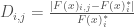
The first metric, regret type 1 (R1), measures a solution’s deviation from its performance in the baseline SOW. Examples of this metric’s use can be found in Kasprzyk et al., (2013) and Lempert and Collins, (2007). As defined by Herman et al., (2015), R1 measures robustness as the 90th percentile deviation in objective performance across SOWs, maximized across all objectives. The 90th percentile is used to capture tail performance while reducing susceptibility to outliers.
Where:
Where represents the value of objective i in the baseline SOW and represents the value of objective i calculated in SOW j.
Below I’ve coded a function which utilizes Rhodium’s built in data structures to calculate R1 for a given solution. The variable results is a Rhodium DataSet object containing the full set of DU reevaluations for one member of the Pareto approximate set. baseline is a DataSet containing the solution’s performance in the baseline state of the world.
def regret_type1(model, results, baseline, percentile=90):
    quantiles = []
    for response in model.responses:
        if response.dir == Response.MINIMIZE or response.dir == Response.MAXIMIZE:
            values = [abs((result[response.name] - baseline[response.name]) / baseline[response.name]) for result in results]
            quantiles.append(np.percentile(values, percentile))

    return max(quantiles)
Regret Type 2
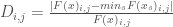
Regret Type 2 (R2), is a variant of Savage regret introduced by Savage, 1951. R2 measures a decision maker’s regret for choosing a given solution over other available solutions by comparing the chosen solution’s performance in each SOW against the best performing option for that SOW. Like R1, R2 utilizes the 90th percentile deviation to capture tail behavior while reducing susceptibility to outliers:
Where:
if objective i is to be minimized and
if objective i is to be maximized.
The best value of each objective i is taken across the set of all solutions s. The deviation in R2 is normalized by the objective value itself rather than the best value, since this objective often approaches zero for minimization problems.
The function below again utilizes Rhodium’s data structures to efficiently implement a function for R2 in python. all_results is a list of DataSet objects, each containing the full set of DU reevaluations for one member of the Pareto approximate set. results is a DataSet containing the full set of DU reevaluations for the member of the Pareto approximate set being evaluated by this function.
def regret_type2(model, all_results, results, percentile=90):
    # for each uncertainty sampling, find the best value
    best = []

    for i in range(len(all_results[0])):
        entry = {}

        for response in model.responses:
            if response.dir == Response.MINIMIZE:
                entry[response.name] = min([result[response.name] for result in all_results])
            elif response.dir == Response.MAXIMIZE:
                entry[response.name] = max([result[response.name] for result in all_results])

        best.append(entry)

    # then compute the regret from the best value
    quantiles = []

    for response in model.responses:
        if response.dir == Response.MINIMIZE or response.dir == Response.MAXIMIZE:
            values = []

            for i in range(len(all_results[0])):
                values.append(abs((results[i][response.name] - best[i][response.name]) / results[i][response.name]))

            quantiles.append(np.percentile(values, percentile))

    return max(quantiles)
Satisficing Type 1
Satisficing metrics quantify a solution’s ability to meet prespecified performance criteria across deeply uncertain SOWs. Satisficing type 1, an approximation of Starr’s domain criterion (Starr 1962; Schneller and Sphicas, 1983) , represents the fraction of states of the world that a solution meets a set of performance criteria.
Where N is the number of sampled SOWs and = 1 if solution s meets the performance criteria in SOW j and = 0 otherwise. For this metric, we’ll utilize the performance criteria stated above: Relibility > 95% and Net Benefit > 0.2.
In python, we can express the performance criteria in a lambda function, as shown in the criteria function defined above. The function below calculates S1 for a solution whose DU reevaluation results have been stored in a DataSet objected called results.
def satisficing_type1(model, results, expr=None):
    # if no criteria are defined, check the feasibility across SOWs
    if expr is None:
        return mean(check_feasibility(model, results))
    # otherwise, return the number of SOWs that meet the specified criteria
    else:
        satisfactory = [expr(result) for result in results]
        return sum(satisfactory)/len(results)
Satisficing Type 2
Satisficing type 2 (S2) is a measure of robustness derived from Info-Gap literature (Ben-Haim, 2004). S2 represents the uncertainty horizon that can be withstood before a solution fails to meet a set of performance criteria.
Where = maximum level of uncertainty, measured outward from the base SOW that can be tolerated before performance drops below threshold r*. In this example, I’ll normalize all uncertainties to their sampling range. In the function below, results is once again a Rhodium DataSet object containing the full set of DU reevaluations for one member of the Pareto approximate set. baseline is a DataSet containing the solution’s performance in the baseline state of the world. uncertainties_min is a list containing the lower bound for each uncertainty and uncertainties_max is a list containing upper bounds.
def satisficing_type2(model, results, baseline, uncertainties_max, uncertainties_min, expr=None):
    distances = []

    # ensure all default parameters are defined in baseline
    baseline = baseline.copy()
    populate_defaults(model, baseline)
    normalized_baseline = [baseline[u.name] for u in model.uncertainties]
    normalized_baseline = (np.array(uncertainties_max)-np.array(normalized_baseline))/(np.array(uncertainties_max)-np.array(uncertainties_min))

    for i, result in enumerate(results):
        if (expr is None and _is_feasible(model, result)) or (expr is not None and expr(result)==False):
            normalized_point = (np.array(uncertainties_max)- np.array([result[u.name] for u in model.uncertainties]))/(np.array(uncertainties_max)-np.array(uncertainties_min))
            distances.append(sp.distance.euclidean(
                    normalized_point,
                    normalized_baseline))

    return 0.0 if len(distances) == 0 else min(distances)
Examining the results
Figure 2: The top ranked solution according to each robustness measure along with each solution’s corresponding ranking across all other measures. Crossing lines indicate contrasting ordinal rankings of solution robustness between two measures. The preferablility of a solution is highly dependent on the choice of robustness metric.
Figure 2 shows the top ranked solution according to each robustness measure along with its corresponding rank across the other three measures. The four measures each provide different rankings of solution robustness. The top ranked solutions for the two regret based measures both preform poorly when evaluated under any of the other three measures, while the best solution according to S1 is tied for the best solution in S2 and ranks in the middle according to the two regret based solution. The second solution selected by S2 ranks at the bottom according to the other three metrics.
The disparity in ranking underscores the differences between the robustness measures. The wide difference in ranking between S2’s best solution and it’s ranking by the other three metrics indicates that while the uncertainties can deviate “far” from the base SOW before this solution fails, its performance is likely to be quite poor once this horizon is crossed. It’s poor ranking in S1 indicates that it will likely fail in many SOWs and it’s R1 ranking suggests that failures in the tail its performance are likely to be quite severe. Finally it’s low ranking in R2 means that there are other solutions that perform better across SOWs.
A solution that performs well by measure S2 may be preferable if decision makers have confidence that their assumptions about the base SOW are correct, however, this is rarely the case in conditions of deep uncertainty, so the solution recommended by S2 alone is likely undesirable. Furthermore, while S2 provides an aggregated measure of “distance to failure” this measure does not indicate which uncertainties drive failure or how far each individual uncertainty must deviate from the base SOW before the solution fails. A better way to understand a solution’s sensitivity to deeply uncertainties is through scenario discovery, which seeks to define vulnerable regions of the uncertainty space for a given solution. Rhodium has a set of built in scenario discovery tools, for details see this post by Julie.
The difference in robustness ranking between measures R1, R2 and S1 leave the decision makers with a choice regarding how they would like a solution to perform. Solutions that perform well in S1 maintain performance across the widest range of potential SOWs, but the metric provides no information on the severity of failure when the criteria is not met. Solutions that perform well in R1 are likely to have the least severe failures in the tails of their performance, but the metric does not measure the fraction of states of the world that result in poor performance. Measure R2 yields information about a solution’s performance relative to other options, but does not provide information about performance criteria or failure severity. As is often the case in decision making problems, the choice of measure should reflect a decision maker’s particular risk tolerance and preferences and must be tailored to each problem individually.
Final thoughts
This example has demonstrated how to use Rhodium to perform the first two steps of MORDM on a four objective formulation of the shallow lake problem. The results indicate that the choice of robustness metric changes which solutions are favored by decision makers. While I’ll wrap up this post here, this should not be the end of an MORDM analysis. After using the robustness metrics to select candidate policies, decision makers should perform scenario discovery to examine which uncertainties control solution performance and how these vulnerabilities differ between candidate solutions. Next, they should visualize each candidate policy to understand how it responds to various system states. Finally, they should think about whether these results necessitate any changes to the original problem formulation. If they choose to reformulate the problem, then the whole process starts back at the beginning. Luckily, Rhodium makes this process easy, allowing decision makers to examine problem formulations quickly and easily.
References
Ben-Haim, Y. (2004). “Uncertainty, probability and information-gaps.” Reliab. Eng. Syst. Saf., 85(1), 249–266.
Carpenter, S.R., Ludwig, D., Brock, W.A., 1999. Management of eutrophication for lakes subject to potentially irreversible change. Ecol. Appl. 9, 751e771.
Groves, D. G., and Lempert, R. J. (2007). “A new analytic method for finding policy-relevant scenarios.” Global Environ. Change, 17(1), 73–85.
Hall, J. W., Lempert, R. J., Keller, K., Hackbarth, A., Mijere, C., and McInerney, D. J. (2012). “Robust climate policies under uncertainty: A comparison of robust decision making and info-gap methods.” Risk Anal., 32(10), 1657–1672
Herman, J.D., Reed, P.M., Zeff, H.B., Characklis, G.W., 2015. How should robustness be defined for water systems planning under change? J. Water Resour. Plan. Manag. 141, 04015012.
Kasprzyk, J. R., Nataraj, S., Reed, P. M., and Lempert, R. J. (2013). “Many objective robust decision making for complex environmental systems undergoing change.” Environ. Modell. Softw., 42, 55–71.
Lempert, R. J., and Collins, M. (2007). “Managing the risk of an uncertain threshold response: Comparison of robust, optimimum, and precaution- ary approaches.” Risk Anal., 27(4), 1009–1026.
Matalas, N. C., and Fiering, M. B. (1977). “Water-resource systems
planning.” Climate, climatic change, and water supply, studies in geo-
physics, National Academy of Sciences, Washington, DC, 99–110.
Quinn, J. D., Reed, P. M., & Keller, K. (2017). Direct policy search for robust multi-objective management of deeply uncertain socio-ecological tipping points. Environmental Modelling & Software, 92, 125-141.
Savage, L. J. (1951). “The theory of statistical decision.” J. Am. Stat. Assoc., 46(253), 55–67.
Schneller, G., and Sphicas, G. (1983). “Decision making under uncertainty: Starr’s domain criterion.” Theory Decis., 15(4), 321–336.
Starr, M. K. (1962). Product design and decision theory, Prentice-Hall, Englewood Cliffs, NJ.
One of my main projects in the last couple years has been in the Upper Colorado River Basin, where we’ve been investigating how hundreds of water users in the basin might be affected by a variety of different changes and uncertainties that might take place in the region. Being in Colorado, water allocation in the basin follows prior-appropriation, where every user has a certain water right, defined by its seniority (where more senior = better) and its decree (i.e. how much water the right is granted for extraction). For the different users in the basin to receive water for their respective uses, prior-appropriation determines who gets X amount of water first based on seniority and given water availability, and then repeats down the seniority order until all requested water has been allocated. Hence, no user can extract water in a manner that affects any senior to them user.
During this investigation, we’ve been interested in seeing how this actually plays out through time and space in the basin, with the aim of potentially better understanding any consequential relationships that might exist between different users, as well as any emerging patterns that might be missed by looking at the data in a different manner. I tried to write a little script to do this in Python. I will be visualizing how users along the basin requested for some water at some historical month (the demand) and how much of that demand was actually met (the shortage), based on their right seniority and water availability in the basin.
There have been multiple posts in the blog on generating maps in Python (as well as in other languages), and they all use a module called Basemap which has been the most popular for these things, but it’s kinda buggy, and kinda a pain to install, and kinda a pain to get working, and I spent the better part of an entire workday to re-set it up on my machine and couldn’t. Enter Cartopy. After Basemap was announced deprecated, Cartopy was meant to be its replacement so I decided to transition. It was super easy to install and start generating maps within a couple minutes and the code I’ll be sharing today will be using that. I will also be using matplotlib’s animation classes to capture the water allocation to the different users through time in a video or a GIF.
First, I load up all necessary packages and data. structures contains the X and Y coordinates of all the diversion points; demands and shortages contain monthly data of water demand and shortage for each diversion point.
import numpy as np
import cartopy.feature as cpf
import cartopy.crs as ccrs
import matplotlib.pyplot as plt
import cartopy.io.img_tiles as cimgt
import pandas as pd
import matplotlib.animation as animation
import math

structures = pd.read_csv('modeled_diversions.csv',index_col=0)
demands = pd.read_csv('demands.csv',index_col=0)
shortages = pd.read_csv('shortages.csv',index_col=0)
Then, I set up the extent of my map (i.e., the region I would like to show). rivers_10m loads the river “feature” at a 10m resolution. There’s a lot of different features that can be added (coastlines, borders, etc.). Finally, I load the tiles which is basically the background map image (many other options also).
I draw the figure more or less as I would in matplotlib, using the matplotlib scatter to draw my demand and shortage points. The rest of the lines are basically legend customization by creating dummy artists to show max demands and shortages in the legend.
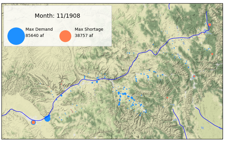
This code should produce something like the following, which shows the relative demand across users in blue, as well as how much of that demand was not met (shortage) in orange for November 1908. The large circles in the legend show the max demand and shortage across all users across all months in the record for reference.
To animate this, it’s very simple. All we need to create is another function (in this case update_points) that will define what changes at every frame of the animation. I’ve defined my function to adjust the size of every circle according to the timestep/frame, as well as change the title of the legend to the correct month. Matplotlib’s FuncAnimation then uses that and my figure to update it repeatedly (in this case for 120 steps). Finally, the animation can be saved to a video.
There’s a lot to be added and improved, but from this simple version we can immediately see certain diversions popping out as well as geographical regions that exhibit frequent shortage. I will continue working on this and hopefully share improved versions in the future.
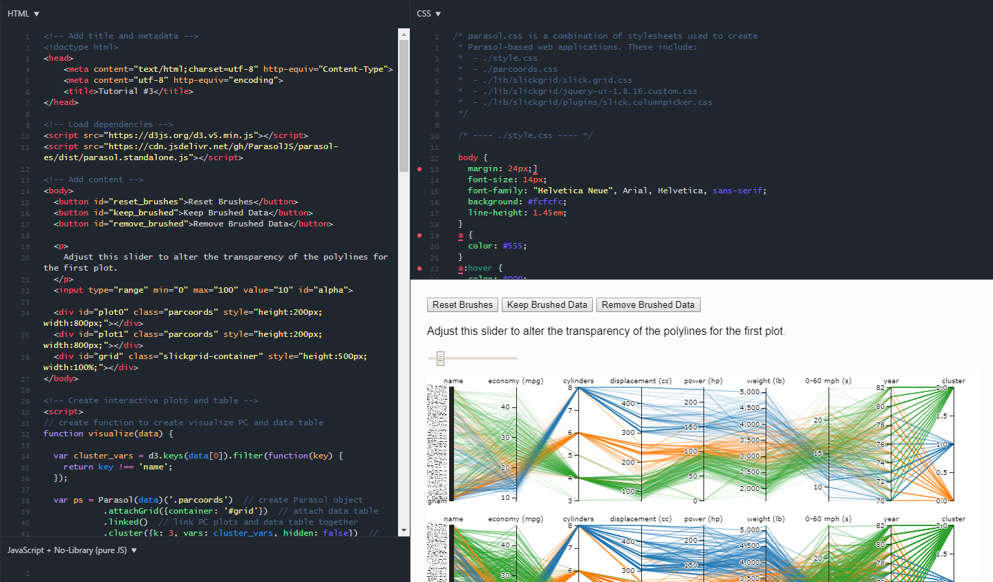
A demonstration of Parasol features like linked plots and data tables, highlighting individual polylines, and brushing and marking data.
In this post, I will describe how to start making your own interactive visualizations with Parasol.
Parasol Wiki
The best place to look for Parasol resources is the wiki page on the GitHub repo. Here you will find the API documentation, an introduction to web development for Parasol, and step-by-step tutorials taking you through the app development process. Because the wiki is likely to grow over time, I won’t provide links to these resources individually. Instead, I’ll give an overview of these resources here but I encourage you to visit the wiki for the most up-to-date tutorials and documentation.
API
The Application Programming Interface (API) is a list of all the features of the Parasol library. If you want to know everything that Parasol can do, the API is the perfect reference. If you are just getting started, however, this can be overwhelming. If that is the case, go through the tutorials and come back to the API page when you want to take your apps to the next level.
Web Development Basics
Creating Parasol apps requires some level of web development knowledge, but to build simple apps, you only need to understand the basics of HTML, JavaScript, and CSS. Check out the web development tutorial on the wiki for an overview of those concepts.
Tutorials
To start developing right away, go through the tutorials listed on the wiki page. These posts take the user through how to create a minimal Parasol app, they touch on the primary features of the API, and more advanced topics like how to use HTML buttons and sliders to create more polished apps.
Creating shareable apps with JSFiddle
Using JSFiddle to create shareable Parasol apps (without having to host them on a website)
I recently discovered JSFiddle–a sandbox tool for learning web development. Not only has JSFiddle made web development more accessible and easier for me to learn, but I realized its a great way to share Parasol apps in an efficient, informal way. Check out the tutorial on the wiki for more details and the following links to my own Parasol “fiddles”:
As I’ve said before, check out Parasol and give us your feedback. If you think this library is valuable, submit an Issue or Star the GitHub repo, or write a comment below. We are open to new ideas and features about how Parasol can better suit the needs of developers.
References
Raseman, William J., Joshuah Jacobson, and Joseph R. Kasprzyk. “Parasol: An Open Source, Interactive Parallel Coordinates Library for Multi-Objective Decision Making.” Environmental Modelling & Software 116 (June 1, 2019): 153–63. https://doi.org/10.1016/j.envsoft.2019.03.005.
Part 2 of our MOEAFramework Training covers the optimization of the lake problem using your choice of algorithms. The relevant files and folders for this part of the training have been added to the Github repo. These are:
lib folder
global.properties
generate_samples.sh
settings.sh
run.sh
algorithm parameter files
In general, the goal of diagnostics is to conduct the optimization of a test problem (the lake problem in our case) using different evolutionary algorithms and to evaluate the performance of these algorithms.
Steps for Optimization
New files and folders:
lib folder: The lib folder contains the Java libraries with source code for the evolutionary algorithms, libraries that may be called from within the algorithms, and a Java version of Borg. Unzip this folder before starting the training.
global.properties: This file is necessary for MOEAFramework to recognize the external problem. Lines 1 and 2 indicate the name of the problem and the class that had been indicated in the lake.java file and the resulting lake.class file.
settings.sh: This file defines the relevant parameters for the optimization.
Line 1 contains the names of the algorithms to be tested.
Line 2 indicates the number of samples of the algorithms that the user wants to test. Each algorithm has a set of parameters that characterize it. These parameters can be anything from population size to crossover rate. Each parameter has an acceptable range of values. In a diagnostics study, it is typical to take multiple Latin Hypercube samples within these ranges to obtain different instances of the algorithm to test.
Line 3 indicates the number of seeds (number of replicate trials)
Line 4 indicates the name of the problem (name of the .class file)
Line 9 shows that the relevant Java files are all in the lib folder
Line 45 is where the user states the epsilons for each objective
Line 50 is where the user specifies the number of functional evaluations
Run this script by typing ./settings.sh
generate_samples.sh: The next step is to generate NSAMPLES of the MOEAs specified in the settings.sh file. In order to do this, you must provide a text file with the relevant parameter ranges for each algorithm. I have added these parameter files for the 5 MOEAs that I have chosen to use, which represent a wide range of different styles and generations of MOEAs, from the older, but most commonly downloaded algorithm, NSGA-II, to some of the newer reference point and reference vector algorithms, NSGA-III and RVEA. These files contain the names of the parameters and the relevant range of values. It is important to note that these parameter ranges might not always be relevant to every problem. Some parameter values depend on the number of objectives and/or decision variables. General rules and defaults for algorithm and operator parameters can be found here and here.
Run this script by typing ./generate_samples.sh
This script utilizes the SampleGenerator from MOEAFramework to produce a corresponding sample file, with each row corresponding to a different parameterization of that algorithm.
run.sh: This bash script is where the meat of the optimization takes place. The script reads in the parameter/sample files and information from the settings.sh file to set up the problem. Then, through a for-loop, the script uses the DetailedEvaluator from MOEAFramework to perform the optimization for all algorithms, seeds, and samples. The arguments for this java command are intuitive- the only unspecified one being the f flag, which states, in this case, that the output be reported every 100 functional evaluations.
Run this script by typing ./run.sh
This script will submit a job for each seed of each algorithm and create a directory called data_raw to store the optimization results. Each job will take up 1 processor. All parameterizations of the algorithm will be running on the same processor. Depending on the complexity of the problem, the number of functional evaluations, and the number of parameterizations, the optimization of the problem could take a very long time. It is important to start off with small trials to understand how a problem scales with increased NFE, parameterizations, and Monte Carlo sampling if that is relevant to your problem. Below is a table outlining some examples of timing trials that one can do to determine problem complexity as well as to determine approximate wall clock time for trials.
No. of Seeds
No. of Parameterizations
No. of MC Samples
NFE
Time
1
1
1000
25,000
16 minutes
1
1
5000
25,000
1 hr, 23 minutes
10
1
1000
25,000
1 hr, 24 minutes
1
2
1000
25,000
32 minutes
10
1
10000
25,000
3 hours
1
100
1000
25,000
25 hours
1
2
1000
200,000
4 hours
This finishes up Part 2 of the MOEAFramework training. In Part 3, we will go over how to evaluate the performance of our algorithms by generating metrics.
Credits: All of the bash scripts in the training repo are written by Dave Hadka, the creator of MOEAFramework.
For my entire graduate student career, I’ve gravitated toward parallel coordinates plots… in theory. These plots scale well for high-dimensional, multivariate datasets (Figure 1); and therefore, are ideal for visualizing multi-objective optimization solutions. However, I found it difficult to create parallel coordinates plots with the aesthetics and features I wanted.
Figure 1. An example parallel coordinates plot that visualizes the “cars” dataset. Each polyline represents the attributes of a particular car and similar types of cars have the same color polyline.
I was amazed when I learned about Parcoords–a D3-based parallel coordinates library for creating interactive web visualizations. D3 (data-driven documents) is a popular JavaScript library which offers developers total control over their visualizations. Building upon D3, the Parcoords library is capable of creating beautiful, functional, and shareable parallel coordinates visualizations. Bernardo (@bernardoct), David (@davidfgold), and Jan Kwakkel saw the potential of Parcoords, each developing tools (tool #1 and tool #2) and additional features. Exploring these tools, I liked how they linked parallel coordinates plots with interactive data tables using the SlickGrid library. Being able to inspect individual solutions was so powerful. Plus, the features in Parcoords like interactive brushing, reorderable axes, easy-to-read axes labels, blew my mind. Working with large datasets was suddenly intuitive!
The potential of these visualizations was inspiring, but learning web development (i.e., JavaScript, CSS, and HTML) was daunting. Not only would I have to learn web development, I would need to learn how to use multiple libraries, and figure out how to link plots and tables together to make these types of tools. It just seemed like too much work for this sort of visualization to catch on… and that was the inspiration behind Parasol. Together with my advisor (Joe Kasprzyk, @jrk301) and Josh Jacobson, we built Parasol to streamline the development of linked, web-based parallel coordinates visualizations.
Raseman, William J., Joshuah Jacobson, and Joseph R. Kasprzyk. “Parasol: An Open Source, Interactive Parallel Coordinates Library for Multi-Objective Decision Making.” Environmental Modelling & Software 116 (June 1, 2019): 153–63. https://doi.org/10.1016/j.envsoft.2019.03.005.
In this post, I’ll provide a brief, informal overview of Parasol’s features and some example applications.
Cleaning up the clutter with Parasol
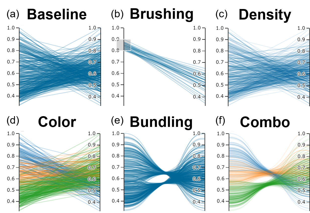
Parallel coordinates can visualize large, high-dimensional datasets, but at times they can become difficult to read when polylines overlap and obscure the underlying data. This issue is known as “overplotting” (see Figure 1 and 2a). That’s why we’ve implemented a suite of “clutter reduction techniques” in Parasol that enables the user to tidy up the data dynamically.
Probably the most powerful clutter reduction technique is brushing (Figure 2b). Using interactive filters, the user can filter out unwanted data and focus on a subset of interest. Users can also alter polyline transparency to reveal density in the data (Figure 2c), assign colors to polylines (Figure 2d), and apply “curve bundling” to group similar data together in space (Figure 2e). These clutter reduction techniques can also be used simultaneously to enhance the overall effect (Figure 2f).
Figure 2. Vanilla parallel coordinates plots (a) suffer from “overplotting”, obscuring the underlying data. Interactive filters (b: brushes) and other clutter reduction techniques (c-f) alleviate these issues.
Another cool feature of both Parcoords and Parasol is dynamically reorderable axes (Figure 3). With static plots, the user can only look at pairwise relationships between variables plotted on adjacent axes. With reorderable axes, they are free to explore any pairwise comparison they choose!
Figure 3. Users can click and drag axes to interactively reorder them.
API resources
The techniques described above (and many other features) are implemented using Parasol’s application programming interface (API). In the following examples (Figures 4-6), elements of the API are denoted using ps.XXX(). For a complete list of Parasol features, check out the API Reference on the Parasol GitHub repo.
Example applications
The applications (shown in Figures 4-6) demonstrate the library’s ability to create a range of custom visualization tools. To open the applications, click on the URL in the caption below each image and play around with them for yourself. Parallel coordinates plots are meant to be explored!
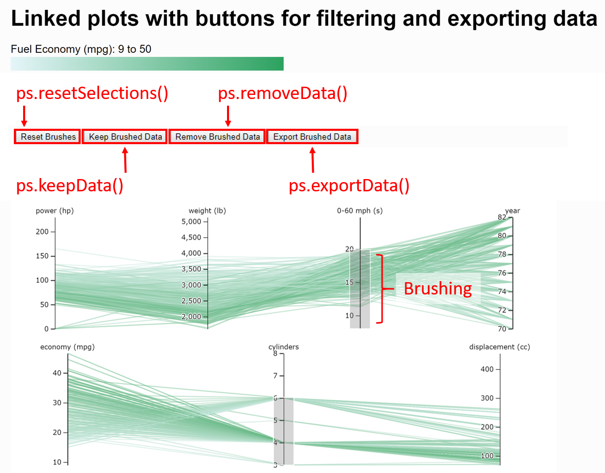
Example app #1 (Figure 4) illustrates the use of linked parallel coordinates plots. If the user applies a brush on one plot, the changes will be reflected on both linked plots. Furthermore, app developers can embed functionalities of the Parasol API using HTML buttons. For instance, if the user applies multiple brushes to the plots, they can reset all the brushes by clicking on the “Reset Brushes” button which invokes ps.resetSelections(). Other functionalities allow the user to remove the brushed data from a plot [ps.removeData()] or keep only the brushed data [ps.keepData()] and export brushed data [ps.exportData()].
Example app #2 (Figure 5) demonstrates utility of linking data tables to parallel coordinates plots. By hovering a mouse over a data table row, the corresponding polyline will become highlighted. This provides the user with the ability to fine-tune their search and inspect individual data points–a rare feature in parallel coordinates visualizations.
App #2 also demonstrates how k-means clustering [ps.cluster()] can enhance these visualizations by sorting similar data into groups or clusters. In this example, we denote the clusters using color. Using a slider, users can alter the number of clusters (k) in real-time. Using checkboxes, they can customize which variables are included in the clustering calculation.
Example app #3 also incorporates clustering but encodes the clusters using both color and “curve bundling”. With curve bundling, polylines in the same cluster are attracted to one another in the whitespace between the axes. Bundling is controlled by two parameters: 1) curve smoothness and 2) bundling strength. This app allows the user to play around with these parameters using interactive sliders.
Similar to highlighting, Parasol features “marking” to isolate individual data points. Highlighting is temporary, when the user’s mouse leaves the data table, the highlight will disappear. By clicking a checkbox on the data table, the user can “mark”data of interest for later. Although marks are more subtle than highlights, they provide a similar effect.
Lastly, this app demonstrates the weighted sum method [ps.weightedSum()]. Although we don’t generally recommend aggregating objectives in multi-objective optimization literature, there are times when assigning weights to different variables and calculating an aggregate score can be useful. In the above example, the user can input different combinations of weights with text input or using sliders.
We want to hear from you!
For the most up-to-date reference on Parasol, see the GitHub repo, and for additional examples, check out the Parasol webpage. We would love to hear from you, especially if you have suggestions for new features or bugs to report. To do so, post on the issues page for the repo.
If you make a Parasol app and want to share it with the world, post a link in the comments below. It would be great to see what people create!
Parasol tutorials
If you aren’t sure how to start developing Parasol applications, don’t worry. In subsequent posts, I’ll take you step-by-step through how to make some simple apps and give you the tools to move on to more complicated, custom applications.
Those tutorials are currently under development and can be found on the Parasol GitHub wiki.
A few years ago, a very dear friend of mine told me about R-Markdown. I was working on a report, and he said that I should try this very cool tool. I did so but not immediately. I started with an “if it ain’t broke, don’t fix it” attitude. However, I quickly realized that R-Markdown really is helpful—well, at least in many situations.
What is R-Markdown? It is a script-based text-development platform for preparing high-quality papers and reports. This strong tool is effective for use on complicated documents that have various types of diagrams and tables. R-Markdown is a distribution of Markdown language for R. More information about Markdown can be found here. Personally, I’ve found R-Markdown to be a powerful tool for creating tutorial documents that include figures, tables, blocks of code, and more. R-Markdown can also be very helpful for working on papers; you can have everything in the same place. For example, as you will see in this tutorial, you can generate your figures and tables within documents. Because it is script-based, R-Markdown is reproducible; you will always get the same text format and figure quality. Therefore, if you want to have a professional-looking CV or are working on a paper or report, I suggest giving R-Markdown a try. The tool might become your new best friend.
install R Markdown
There are two steps to install R-Markdown:
1- Install R Markdown
# 1- Install R Markdown

install.packages("rmarkdown")
library(rmarkdown)
2- You also need to install “tinytex”. You can use the following command to install and load “tinytex”
tinytex::install_tinytex()
library(tinytex)
Create an R-Markdown Document
To create your first R-Markdown document, start by installing R-Markdown. Then, open the “File” menu, and click on “New File.” From the dropdown menu, select “R-Markdown.” Doing so will open an R-Markdown file in your RStudio. The file comes with very simple and informative instructions.
On a side note, I use RStudio, which is a popular and user-friendly integrated development environment (IDE) for R. You can find more information about it (here).
Publish your document
The final format of your output document can be pdf, html, or word. To select your favorite output and generate your final document, click on “Knit,” which opens a dropdown menu. Select the output format—for example, pdf—and it will generate your document.
Components of an R-Markdown Code
R-Markdown documents usually include meta-data, text, and code chunks. The following sections briefly describe the components, and more information can be found on R-Markdown’s website.
Meta-Data
When generating documents, R-Markdown requires some initial information and instructions. These can include general data about the documents—for example, date, title, output format, and author’s name.
Text
Text parts in R-Markdown follow the tradition of other document-markup languages such as LaTex (see here). However, R-Markdown is easier than LaTex. Basically, authors can use scripts to adjust document formatting. Many details can be listed about R-Markdown’s text-formatting commands, but I am not going to explain them in this short tutorial. These cheat sheets here and here provide enough information to get you started on writing an R-Markdown document. A few examples: #header creates headers, ‘[]()’ creates a hyperlink. You can use $ to insert equations (e.g. $y=ax^{2}+ bx +c$).
Code Chunks
Different types of code chunks can be used in R-Markdown; the types depend on application of the code. You might want to show your code when you develop an instruction. You can also write a code solely for generating a figure, but you may not want to show the code itself. The following is a generated timeline figure of Michael Jackson’s life; you can see the code.
#You need to uncomment ``` lines

#```{r timeline}

# This code chunck generates a timeline of Michael Jackson life.

library(timelineS)
timelineS(mj_life, main = "Life of Michael Jackson",label.cex =   0.7)

#```
Adding Tables
There are different libraries available in R for generating nice-looking tables. Here I use knitr.
#You need to uncomment ``` lines

#```{r table}

library(ggplot2)

library(knitr)
kable(mpg[1:8,])

#```
Adding Figures to Your Document
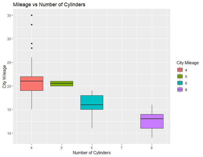
R-Markdown allows you to generate plots in your documents. For example, you can use ggplot, which is a powerful figure-creation library in R, to create and insert a plot into your document. See the following. If you include echo = FALSE to the header of your code chunk, the code would disappear on your final pdf file.
#You need to uncomment ``` lines

#```{r ggplot}

library(ggplot2)

# MPG dataset is already available in ggplot2, I use it to generate the following figure

ggplot(mpg, aes(x=cyl, y=cty)) + geom_boxplot(aes(fill=factor(cyl))) +
    labs(title="Mileage vs Number of Cylinders",
         x="Number of Cylinders",
         y="City Mileage",
         fill="City Mileage")

#```
TLDR; Python script for radial convergence plots that can be found here.
You might have encountered this type of graph before, they’re usually used to present relationships between different entities/parameters/factors and they typically look like this:
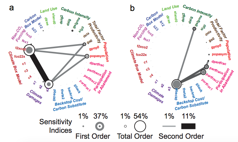
In the context of our work, I have seen them used to present sensitivity analysis results, where we are interested in both the individual significance of a model parameter, but also the extent of its interaction with others. For example, in Butler et al. (2014) they were used to present First, Second, and Total order parameter sensitivities as produced by a Sobol’ Sensitivity Analysis.
From Butler et al. (2014)
I set out to write a Python script to replicate them. Calvin Whealton has written a similar script in R, and the same functionality also exists within Rhodium. I just wanted something with a bit more flexibility, so I wrote this script that produces two types of these graphs, one with straight lines and one with curved (which are prettier IMO). The script takes dictionary items as inputs, either directly from SALib and Rhodium (if you are using it to display Sobol results), or by importing them (to display anything else). You’ll need one package to get this to run: NetworkX. It facilitates the organization of the nodes in a circle and it’s generally a very stable and useful package to have.
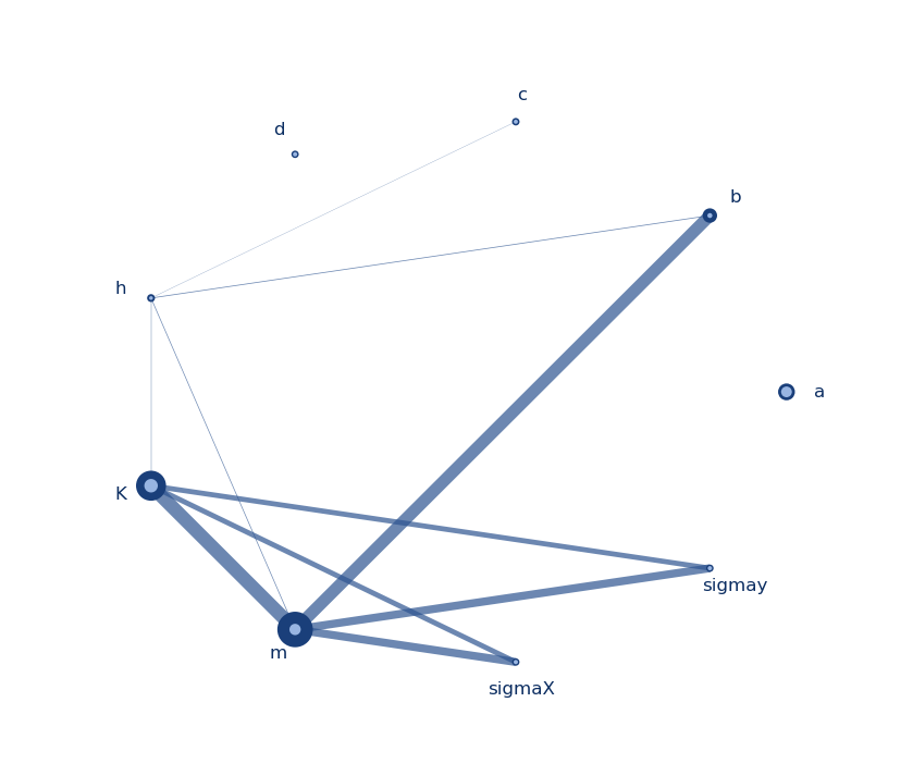
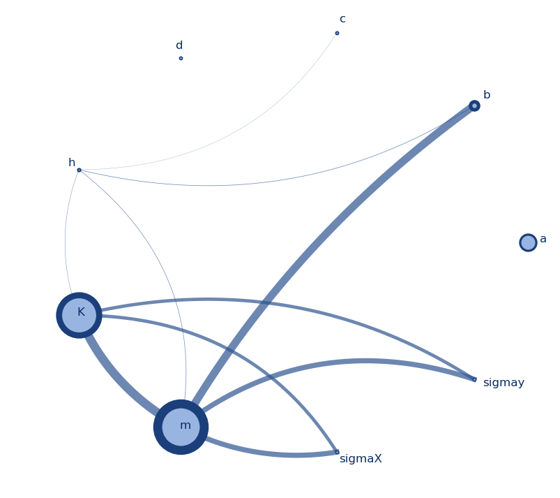
Graph with straight linesGraph with curved lines
I made these graphs to display results the results of a Sobol analysis I performed on the model parameters of a system I am studying (a, b, c, d, h, K, m, sigmax, and sigmay). The node size indicates the first order index (S1) per parameter, the node border thickness indicates the total order index (ST) per parameter, and the thickness of the line between two nodes indicates the secord order index (S2). The colors, thicknesses, and sizes can be easily changed to fit your needs. The script for these can be found here, and I will briefly discuss what it does below.
After loading the necessary packages (networkx, numpy, itertools, and matplotlib) and data, there is some setting parameters that can be adapted for the figure generation. First, we can define a significance value for the indices (here set to 0.01). To keep all values just set it to 0. Then we have some stylistic variables that basically define the thicknesses and sizes for the lines and nodes. They can be changed to get the look of the graph to your liking.
# Set min index value, for the effects to be considered significant
index_significance_value = 0.01
node_size_min = 15 # Max and min node size
node_size_max = 30
border_size_min = 1 # Max and min node border thickness
border_size_max = 8
edge_width_min = 1 # Max and min edge thickness
edge_width_max = 10
edge_distance_min = 0.1 # Max and min distance of the edge from the center of the circle
edge_distance_max = 0.6 # Only applicable to the curved edges
The rest of the code should just do the work for you. It basically does the following:
Define basic variables and functions that help draw circles and curves, get angles and distances between points
Set up graph with all parameters as nodes and draw all second order (S2) indices as lines (edges in the network) connecting the nodes. For every S2 index, we need a Source parameter, a Target parameter, and the Weight of the line, given by the S2 index itself. If you’re using this script for other data, different information can fit into the line thickness, or they could all be the same.
Draw nodes and lines in a circular shape and adjust node sizes, borders, and line thicknesses to show the relative importance/weight. Also, annotate text labels on each node and adjust their location accordingly. This produces the graph with the straight lines.
For the graph with the curved lines, define function that will generate the x and y coordinates for them, and then plot using matplotlib.
I would like to mention this script by Enrico Ubaldi, based on which I developed mine.


 ,
,  and
and  are the centers, radii and wights of n cubic radial basis functions. These parameters will be the decision variables for our multi-objective optimization (searching for parameters to a rule system like this is known as direct policy search (DPS)). For this example we’ll use n=2 cubic radial basis functions and have 6 decision variables.
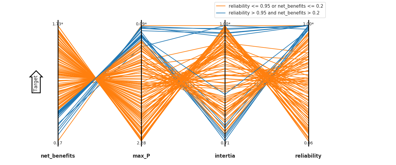
![R1 = \max_i[D_{i,90}:P(D_i\leq D_{i,90}=0.90]](https://s0.wp.com/latex.php?latex=R1+%3D+%5Cmax_i%5BD_%7Bi%2C90%7D%3AP%28D_i%5Cleq+D_%7Bi%2C90%7D%3D0.90%5D&bg=ffffff&fg=444444&s=0&c=20201002)
 represents the value of objective i in the baseline SOW and
  represents the value of objective i calculated in SOW j.
 ![R2 = \max_i[D_{i,90}:P(D_i\leq D_{i,90}=0.90]](https://s0.wp.com/latex.php?latex=R2+%3D+%5Cmax_i%5BD_%7Bi%2C90%7D%3AP%28D_i%5Cleq+D_%7Bi%2C90%7D%3D0.90%5D&bg=ffffff&fg=444444&s=0&c=20201002)


 = 1 if solution s meets the performance criteria in SOW j and
 ![S2 = \hat{\alpha} = max \big[\alpha:min_{j \in U(\alpha)} F(x)_j \geq r^* \big]](https://s0.wp.com/latex.php?latex=S2+%3D+%5Chat%7B%5Calpha%7D+%3D+max+%5Cbig%5B%5Calpha%3Amin_%7Bj+%5Cin+U%28%5Calpha%29%7D+F%28x%29_j+%5Cgeq+r%5E%2A+%5Cbig%5D&bg=ffffff&fg=444444&s=0&c=20201002)
 = maximum level of uncertainty, measured outward from the base SOW that can be tolerated before performance drops below threshold r*. In this example, I’ll normalize all uncertainties to their sampling range. In the function below, results is once again a Rhodium DataSet object containing the full set of DU reevaluations for one member of the Pareto approximate set. baseline is a DataSet containing the solution’s performance in the baseline state of the world. uncertainties_min is a list containing the lower bound for each uncertainty and uncertainties_max is a list containing upper bounds.