Continuous Deployment with GitHub Actions (or, What Gives Life to a Living eBook?)

Continuous Deployment with GitHub Actions (or, What Gives Life to a Living eBook?)

Last month we introduced our free eBook Addressing Uncertainty in MultiSector Dynamics Research. Did you know that, to date, we have published 74 revisions? Without an automated release and deployment process, this would have been very tedious! But, with the help of GitHub Actions, every small edit, minor clarification, or major improvement can go live within moments of merging the code. Read on to learn how the eBook team leverages GitHub Actions for CI/CD (Continuous Integration / Continuous Delivery).

GitHub Workflow

A reliable CI/CD strategy depends on a robust code review process⁠—continuously delivering bugs and typos will not impress anyone! There are many acceptable workflows; the best one to use will depend on team composition and codebase. In our case, a feature branching workflow suffices:

Feature Branching Workflow

The feature branching workflow consists of a main code branch representing published assets. New features or bug fixes require authors to create a new branch from main, implement their changes, and then submit a pull request back into main. A pull request is a formal code review process that gives other authors a chance to provide feedback on the proposed changes. Once consensus has been reached, the feature branch is merged into the main branch, kicking off the CI/CD process.

Automation

While the code review process is designed to catch content and conceptual errors, subtle process and system based errors can often slip through the cracks. Thus the first step in the CI/CD process should be running a suite of automated tests that span a range of systems, behaviors, and any known pain points. The depth and breadth of these tests should be sufficient to ensure an adequate degree of publication readiness without being overly burdensome to maintain. The test suite can grow over time!

For the eBook, our tests simply ensure that the Python dependencies install correctly on Linux, Mac, and Windows containers, that the supporting code can be imported on these systems without error, and that the HTML and PDF versions of the publication generate successfully. If any tests fail, the publication process is cancelled and the authors are notified with details of the failure.

This test, release, and publication process is orchestrated by GitHub Actions. Read on to learn more!

GitHub Actions

GitHub Actions are available to any project hosted in GitHub—totally free for public repositories, and free to a limited extent for private repositories. An Action can be defined as a unit of work performed using a virtual machine in response to an event. In GitHub, Actions are defined using YAML files places into the .github/workflows directory of a repository. YAML (YAML Ain’t Markup Language) is a concise, human-readable syntax for conveying semi-structured data. The minimal content of a GitHub Action includes a name, one or more event triggers, and one or more jobs. A job consists of a name, one or more virtual machine targets, and one or more steps. For example, the eBook test Action looks like this:

.github/workflows/01_test.yml
name: Test
on:
  push:
    branches: [ main ]
jobs:
  test:
      runs-on: ${{ matrix.os }}
      strategy:
        matrix:
          os: [ubuntu-latest, macos-latest, windows-latest]
      steps:
        - uses: actions/checkout@v2
        - name: Set up Python
          uses: actions/setup-python@master
          with:
            python-version: 3.9
        - name: Install dependencies
          run: |
            python -m pip install --upgrade pip
            pip install -r requirements.txt
        - name: Run tests
          run: |
            pip install pytest
            pytest

There is a lot going on here, so let’s take it step by step!

name: Test
on:
  push:
    branches: [ main ]

This snippet gives our Action a name, and specifies that it should trigger on updates to the main branch of the repository.

jobs:
  test:
      runs-on: ${{ matrix.os }}
      strategy:
        matrix:
          os: [ ubuntu-latest, macos-latest, windows-latest ]

This snippet defines a job within our “Test” Action named “test”, and then uses special syntax to declare that the job should be run on three different virtual machines: the latest Ubuntu Linux, macOS, and Windows containers. Running the tests on multiple operating systems helps catch bugs with system-specific dependencies.

      steps:
        - uses: actions/checkout@v2
        - name: Set up Python
          uses: actions/setup-python@master
          with:
            python-version: 3.9
        - name: Install dependencies
          run: |
            python -m pip install --upgrade pip
            pip install -r requirements.txt
        - name: Run tests
          run: |
            pip install pytest
            pytest

This snippet outlines the actual units of work within the job; each “-” separates a unique task. The uses syntax is special in that it allows one to leverage tasks written by others hosted in the GitHub Actions Marketplace. The actions/checkout@v2 task clones the repository onto the virtual machine, and the actions/setup-python@master task installs and configures the specified Python version. The final two steps use the run directive to invoke custom code, in this case installing Python dependencies and running the Python test suites.

Deployment

Once the tests successfully pass, it’s time to publish! Since the eBook is essentially a web app, GitHub Pages is the perfect deployment platform. Pages hosts the content of a branch as a website, and is free for public repositories.

If you followed along with the previous eBook post, you learned about the Python, Sphinx, and Restructured Text workflow for compiling the eBook content into a polished product. Let’s create a GitHub Action to compile the eBook and deploy it to GitHub Pages! Here’s the full YAML file:

.github/workflows/02_deploy.yml
name: Deploy
on:
  push:
    branches: [ main ]
jobs:
  build:
    runs-on: ubuntu-latest
    steps:
      - uses: actions/checkout@v2
      - uses: actions/setup-python@v2
        with:
          python-version: '3.9'
      - name: Install latex dependencies
        run: sudo apt-get update -y && sudo apt-get install -y texlive latexmk texlive-latex-recommended texlive-latex-extra texlive-fonts-recommended ghostscript
      - name: Update pip and install python dependencies
        working-directory: 'docs/'
        run: |
          python -m pip install --upgrade pip
          pip install -r requirements.txt
      - name: Build html and pdf ebook
        working-directory: 'docs/'
        run: |
          make html latexpdf --keep-going LATEXMKOPTS="-interaction=nonstopmode" || true
          make latexpdf --keep-going LATEXMKOPTS="-interaction=nonstopmode" || true
          make latexpdf --keep-going LATEXMKOPTS="-interaction=nonstopmode" || true
        continue-on-error: true
      - name: Get current datetime in ISO format
        id: date
        run: echo "::set-output name=date::$(date -u +'%Y-%m-%d')"
      - name: Create GitHub release
        id: gh_release
        uses: softprops/action-gh-release@v1
        with:
          files: docs/build/latex/addressinguncertaintyinmultisectordynamicsresearch.pdf
          tag_name: ${{ steps.date.outputs.date }}v${{ github.run_number }}
      - name: Commit the compiled files
        run: |
          cd docs/build/html
          git init
          git add -A
          git config --local user.email "action@github.com"
          git config --local user.name "GitHub Action"
          git commit -m 'deploy' -a || true
      - name: Push changes to gh-pages
        uses: ad-m/github-push-action@master
        with:
          branch: gh-pages
          directory: docs/build/html
          force: true
          github_token: ${{ secrets.GITHUB_TOKEN }}

A lot to unpack here! Let’s take it step by step. As before, we start by naming the Action, triggering it on updates to the main branch, declaring that it should run only on an ubuntu-latest virtual machine, checking out out the code, and setting up Python. Then we get into the new job steps:

      - name: Install latex dependencies
        run: sudo apt-get update -y && sudo apt-get install -y texlive latexmk texlive-latex-recommended texlive-latex-extra texlive-fonts-recommended ghostscript

This step installs all the operating system dependencies needed to support the Latex syntax and compilation to PDF. There was some trial and error involved in getting this right, but once correct it should be pretty stable.

      - name: Build html and pdf ebook
        working-directory: 'docs/'
        run: |
          make html latexpdf --keep-going LATEXMKOPTS="-interaction=nonstopmode" || true
          make latexpdf --keep-going LATEXMKOPTS="-interaction=nonstopmode" || true
          make latexpdf --keep-going LATEXMKOPTS="-interaction=nonstopmode" || true
        continue-on-error: true

This step runs the Sphinx makefile to compile the HTML and PDF versions of the eBook. The verbosity and repetitiveness of these commands works around some unusual oddities of the Latex and PDF compilation. --keep-going LATEXMKOPTS="-interaction=nonstopmode" prevents the command from waiting for user input. || true and the repeated make latexpdf lines allow the PDF engine to fully resolve all the references in the restructured text files; otherwise the PDF file would be incomplete and garbled (this one stumped us for awhile!).

      - name: Get current datetime in ISO format
        id: date
        run: echo "::set-output name=date::$(date -u +'%Y-%m-%d')"
      - name: Create GitHub release
        id: gh_release
        uses: softprops/action-gh-release@v1
        with:
          files: docs/build/latex/addressinguncertaintyinmultisectordynamicsresearch.pdf
          tag_name: ${{ steps.date.outputs.date }}v${{ github.run_number }}

To make it easier to chronologically place our eBook releases, we wanted to include a date stamp in our version tags. The first step above assigns the date to a variable. The second step above creates and tags an official GitHub release (using the date and an auto-incrementing run number), and includes the PDF version of the eBook as an asset attached to the release.

      - name: Commit the compiled files
        run: |
          cd docs/build/html
          git init
          git add -A
          git config --local user.email "action@github.com"
          git config --local user.name "GitHub Action"
          git commit -m 'deploy' -a || true
      - name: Push changes to gh-pages
        uses: ad-m/github-push-action@master
        with:
          branch: gh-pages
          directory: docs/build/html
          force: true
          github_token: ${{ secrets.GITHUB_TOKEN }}

These two steps cause the GitHub Actions user to commit the compiled HTML files and force push them to the gh-pages branch of our repository, using a secret token. This is a common “hack” to enable publishing only the desired web assets and not the entire repository. Never force push to other shared code branches!

Action Status

Check the status of the CI/CD pipeline using the Actions tab of the GitHub repository. Successful Actions show a check mark, in progress Actions show a spinner, and failed Actions show an X. Clicking into a particular Action will show more details, log messages, and error traces if relevant.

The GitHub Actions Tab

Slack Integration

To take our workflow to the next level (and to avoid the need to read even more email 😅 ), we added the GitHub app to our eBook Slack channel. This adds a bot that can subscribe to GitHub repositories and report on activity; for instance: new issues, new pull requests, and new releases. We can then discuss and iterate inline in Slack, without having to jump to other apps or sites.

GitHub Slack Integration

To add the GitHub bot to a channel, right click on the channel name, select “Open channel details”, and navigate to the “Integrations” tab. From here, you can choose “Add apps” and search for GitHub. Once added, type a bot command such as /github subscribe [repository name] to start receiving notifications in the channel. The bot can also be used to open and close issues!

Conclusion

Using the GitHub Actions workflow to automate the testing and publication of our eBook enabled our team to focus more on the content and quality of release rather than stumbling over the intricacies of the publication process. CI/CD has been a powerful tool in software communities, but can greatly benefit researchers and academics as well. We hope our learnings presented above will speed you along in your own workflows!

Efficient Storage and Querying of Geospatial Data with Parquet and DuckDB

This post is dedicated to Chris Vernon and Travis Thurber from PNNL who taught me how to use these tools!

Lately, I’ve been generating synthetic weather scenarios for basins in California. The weather scenarios are created at a daily time step and are informed by tree-ring products which span across 600 years. We want to develop multiple ensembles of these scenarios that are representative of plausible future climate changes that the region could experience. It became clear to me that I would need to make sure that I was storing data efficiently and that I was able to parse through these data quickly to generate plots and develop metrics.

Below, I wanted to discuss two points that have really helped my workflow: (1) focusing on file structure and compression and (2) changing the way that I explore the resulting scenarios.

File choice and compression

To illustrate the importance of considering how you choose to save your data, I grab the historical trace of daily precipitation over the last 50 years for the Tuolumne River Basin and upload it into R as a dataframe. Below I show the code to take this dataframe and save it in various formats.

#Traditional RDS
system.time(saveRDS(prcp_tuolumne,"E:/blog/prcp_tuolumne.rds"))

#Compressed RDS
system.time(saveRDS(prcp_tuolumne,"E:/blog/prcp_tuolumne_compressed.rds",compress = 'xz'))

#Text 
system.time(write.table(prcp_tuolumne,"E:/blog/prcp_tuolumne.txt"))

#CSV
system.time(write.csv(prcp_tuolumne,"E:/blog/prcp_tuolumne.csv"))

#Parquet
library(arrow)
system.time(write_parquet(prcp_tuolumne,"E:/blog/prcp_tuolumne.parquet",compression = "gzip"))

#HDF5 
library(rhdf5)
system.time(h5write(prcp_tuolumne,"E:/blog/prcp_tuolumne.h5","df"))


#NetCDF
library(ncdf4)
# path and file name, set dname
ncpath <- "E:/blog/"
ncname <- "prcp_tuolumne"  
ncfname <- paste(ncpath, ncname, ".nc", sep="")
dname <- "prcp"  # note: tmp means temperature (not temporary)
timedim <- ncdim_def("time","days since 1950-11-1",as.numeric(dates))
# define variables
fillvalue <- 1e32
dlname <- "observed precipitation"
prcp_def <- ncvar_def("prcp","mm",list(timedim),1e32,"observed prcp",prec = "double")
# create netCDF file and put arrays
ncout <- nc_create(ncfname,list(prcp_def),force_v4=TRUE)
# put variables
system.time(ncvar_put(ncout,prcp_def,as.matrix(prcp_tuolumne[ ,1])))

Here, I summarize the resulting size and write times for each format.

File TypeSize (Kb)Writing Time (seconds)
RDS9,0652.13
Compressed RDS4,01217.73
HDF55,204323.03
Text26,85112.69
CSV27,02412.14
netCDF141,3603.12
Parquet8,3960.98

Note that the original file size was on the smaller side so this exercise may seem trivial, but when you are creating many ensembles of both precipitation and temperature, across hundreds of years, across may basins, across many climate change scenarios, small files will add up and can potentially limit the scope of experiment that you can conduct if you don’t have enough file storage. Of these file types, one of my recent favorites has been Apache Parquet. Parquet is an open-source column-oriented format that is specifically designed for efficient storage and accessibility of data. Whereas the compressed RDS file and HDF5 beat Parquet in terms of size, it takes much longer to write to these files and subsequently read them back in. Another advantage of Parquet is that it is recognized by common coding languages (R, Matlab, Python) which allows for a more seamless workflow between models of different languages. If you have a little more storage to work with, Parquet is a good choice to balance size and writing time tradeoffs.

Querying data with SQL and DuckDB

Once your data are in an efficient format like Parquet, the next order of business is to make sure that you can easily sort through it and, as Chris would say, “talk to your data and let it talk back”. One way to communicate with your data and ask questions in a more semantically meaningful way is to use Structured Query Language (SQL). There are many methods of querying in R, but a useful data management tool that I have enjoyed interacting with is DuckDB which is a relational database management system. DuckDB has an R API and allows you to use the SQL syntax to query data in an efficient way. It should be noted that you can perform similar aggregation and subsetting using other R base functions, but DuckDB allows you to perform these tasks faster and across multiple files that you may have in a directory.

Let’s use a case where you have developed 30 traces of daily basin-averaged synthetic precipitation for the Tuolumne based on the historical period and each trace is stored in a respective parquet file (“ensemble1.parquetgzip, ensemble2.parquetgzip…ensemble30.parquetgzip). Each ensemble looks something like this:

Example of the parquet file structure

Now let’s state a question that I want to ask to the data and see how to structure these questions using SQL and DuckDB.

“Hey DuckDB, can you create a dataframe for me that provides an annual average across all my synthetic traces? Let’s plot that with respect to the observed annual average and show the bounds of the synthetic traces.”

First we need to open a connection to DuckDB. Then we are going to have to create annual averages from the daily historical and synthetic traces and then create max/min bounds to show the additional variability we are getting from the generator.

In order to answer this question, DuckDB will query all our parquet files simultaneously (!) and return a dataframe with annual averages and we can do some clever sub-querying to get the max/min of the averages. I really enjoy that I don’t have to read in the files into my R workspace. R reads in files and stores them based on memory, so those of you who have used larger datasets might have found that you are limited in how many datasets you can have open, which can be frustrating! This is not an issue with DuckDB.

#Historical trace 
historical=data.frame(dates.year,dates.month,dates.day,rowMeans(prcp_sacsma))
historical_yearly=aggregate(historical,by=list(dates.year),FUN=mean)

# open connection to DuckDB
con <- dbConnect(duckdb::duckdb())

# query to find annual average across all synthetic traces
df=dbGetQuery(con, 
              "SELECT year,
           AVG(precipitation) AS yearly_average
           FROM 'E:/NHMM/blog/*.parquet'
           GROUP BY year
           ORDER BY year")

#For the max/min, we need to find the average first and then return the max/min values in something like a nested approach 

#First create a dataframe with all files 
all_files=dbGetQuery(con,"SELECT *
                FROM 'E:/NHMM/blog/*.parquet'")

# register the dataset as a DuckDB table, and give it a name
duckdb::duckdb_register_arrow(con, "all_files_table", all_files)


annual_average=dbGetQuery(con, 
               "SELECT year,
           AVG(precipitation) AS yearly_average
           FROM all_files_table
           GROUP BY year,sample
           ORDER BY year")

# register the dataset as a DuckDB table, and give it a name
duckdb::duckdb_register_arrow(con, "annual_table", annual_average)

#query to find max
max=dbGetQuery(con, 
               "SELECT year,
           MAX(yearly_average) AS max_yearly_average
           FROM annual_table
           GROUP BY year
           ORDER BY year")

#query to find min
min=dbGetQuery(con, 
               "SELECT year,
           min(yearly_average) AS min_yearly_average
           FROM annual_table
           GROUP BY year
           ORDER BY year")
#Plot the results!
library(ggplot2)

ggplot(df, aes(x = year, y = yearly_average)) +
  geom_ribbon(aes(ymin = min$min_yearly_average,
                  ymax = max$max_yearly_average),
              alpha = 0.2,fill="blue") +
  geom_line()+geom_line(color="blue",size=2)+ geom_line(data=basin.wide.yearly[3:64,],aes(x=year,y=precipitation), color="Black",size=2)+ ggtitle("Annual Average Precipitation") +
  xlab("Year") + ylab("Annual Average Precipitation (mm)")+theme_ridges()

Here’s the resulting figure:

Synthetic generation in blue compared to the historical trace in black

“Hey DuckDB, from all of the synthetic traces that I have generated, how many instances are there where we are producing daily precipitation that is above 10 mm for specifically the years 1980 or 2000?”

In order to answer this question, DuckDB will once again query all our parquet files simultaneously and return a dataframe with all the instances of >10 mm and only for the years 1980 or 2000. This is how you would write this question in “code”.

library(arrow)
library(duckdb)
library(fs)
library(tidyverse)
library(DBI)
library(glue)

# open connection to DuckDB
con <- dbConnect(duckdb::duckdb())

df=dbGetQuery(con,"SELECT *
                FROM 'E:/blog/*.parquet'
                WHERE precipitation > 10
                AND (year = 1980 OR year = 2000)
                order BY year")

If we look at the size of the resulting dataframe it looks like we have generated 1335 instances of daily precipitation that are greater than 10 mm in specifically the years 1980 or 2000:

Hey DuckDB, I want to think about meteorological drought. In how many instances am I half a standard deviation below the long-term average monthly precipitation?

To try this out, let’s just look at one synthetic trace. First we need to find the long term average across the trace and let’s plot what a drought might look like.

# query to grab the first synthetic trace
scenario1=dbGetQuery(con, 
              "SELECT month,year,
           AVG(precipitation) AS monthly_avg
           FROM 'E:/NHMM/blog/ensemble1.parquet'
           GROUP by year, month")

# query to find mean
long_term_average=dbGetQuery(con, 
              "SELECT AVG(precipitation) AS monthly_avg
           FROM 'E:/NHMM/blog/ensemble1.parquet'") 

# query to standard deviation
stdev=dbGetQuery(con, 
              "SELECT AVG(precipitation) AS monthly_stdev
           FROM 'E:/NHMM/blog/ensemble1.parquet'")

We can then plot the synthetic trace (blue), mean (black), and a 1/2 standard deviation (dashed line) below the mean.

Now we can count the number of months that we are classified in a drought across the synthetic trace. Based on the stats that we calculated in the last block, I hard coded in the drought threshold, but in theory, you can nest many functions with more complicated sub-queries.

# register the dataset as a DuckDB table, and give it a name
duckdb::duckdb_register_arrow(con, "scenario_1", scenario1)


instances=dbGetQuery(con, 
                     "SELECT month,year
           FROM scenario_1
           WHERE monthly_avg < 3.125291
           GROUP by year, month
           ORDER by year,month")

It looks like 115/325 months or about 35% of the time we are in a drought in this particular synthetic trace. Yikes! But it makes for a good way to assess the vulnerability of the system to future plausible meteorological drought conditions.

I hope that these approaches can be as useful to you as they have been for me!

Tips for Creating Watershed Maps in R

There have been a few posts on this blog on creating watershed maps (here, here, and here), but this post is going to be focused on some of my recent experiences on creating watershed maps in R with files that may be missing attributes, are in the wrong projection, and contain data that need to be clipped to a specific boundary shapefile. There are lots of packages that exist to do one or more of these things, but anyone who has ever tried to create watershed maps in R knows that there isn’t one package that does it all. My main goal for this post is to outline the most efficient workflow and use of packages that also allow for the most compatibility when plotting shapefiles and raster files in one figure.

In this post, we are going to be creating a map of the Tuolumne River Basin boundary and plot elevation data within the basin. All the data are found here. First we will read in the Tuolumne boundary shape file (.shp) and the elevation raster file (.asc which is an ASCII file) using the appropriate functions and do some preliminary plotting to see what we have.

#Import libraries 

library(rgdal)
library(ggplot2)
library(raster)

#Read in Tuolumne shapefile

tuolumne.basin <- readOGR(dsn = "doi_10.6071_M3FH3D__v5/tuolumne_merced_data_2009-2015/Merced_Tuolumne_Dataset_SpatialData/SpatialData/Tuolumne_utm.shp")

#Read in elevation raster

elevation.raster = raster("doi_10.6071_M3FH3D__v5/tuolumne_merced_data_2009-2015/Merced_Tuolumne_Dataset_SpatialData/SpatialData/merced_tuolumne_100mdem_utm.asc")

#Plot the files
 
ggplot() +  geom_polygon(data = tuolumne.basin, aes(x = long, y = lat, group = group), colour = "dark red", fill = NA)
plot(elevation.raster)
Raw shapefile and raster data

So we have the pieces that we need to build the map, but notice that the latitude and longitude are in the wrong projection. We can use the following command to check what projection the shapefile is in:

proj4string(tuolumne.basin) 

We see that the output is: “+proj=utm +zone=11 +datum=NAD83 +units=m +no_defs”. So we are in the Universal Transverse Mercator coordinate system, but we should change to WGS 84. We can do this using the function “spTransform” which will swap out the projection by adjusting the CRS (Coordinate Reference System) attribute of the shapefile. You can use “proj4string” to verify that the transformation took place.

 tuolumne.basin.transformed <- spTransform(tuolumne.basin, CRS("+proj=longlat +ellps=WGS84 +datum=WGS84"))

Now we need to transform the raster files coordinates. Note that the raster file doesn’t have an associated coordinate reference system listed. If you try to change the projection at this point, you will get an error. This is a minor inconvenience since we know that the coordinate system should match that of the raw Tuolumne shapefile and we can just insert the original coordinate system as a string under the projargs attribute. Then we can transform it to match the coordinate system of the transformed shapefile using “projectRaster”.

elevation.raster@crs@projargs <- "+proj=utm +zone=11 +datum=NAD83 +units=m +no_defs" 
  
elevation.raster.transformed <- projectRaster(elevation.raster,crs=crs(tuolumne.basin.transformed))

Great, now we have all the data in the right projection. Now we have to clip the raster layer to show only the data in the bounds of our shapefile. We first use the “crop” function in the raster library to clip the layer based on the extent of the shapefile boundary as well as the mask function. It is important to do both otherwise the clip will not work!

elevation.raster.transformed.cropped <- crop(elevation.raster.transformed, extent(tuolumne.basin.transformed))
elevation.raster.transformed.cropped <- mask(elevation.raster.transformed, tuolumne.basin.transformed)

Now we need to get the appropriate elevation values and coordinates from the raster object so that we can plot it using ggplot.When we use ggplot here, notice that we only need to use geom_raster and elevation data since the clipped data will perfectly follow the shapefile boundary.

#Isolate elevation values from the raster file

val <- getValues(elevation.raster.transformed.cropped)
xy <-as.data.frame(xyFromCell(elevation.raster.transformed.cropped,1:ncell(elevation.raster.transformed.cropped)))
xy <- cbind(xy,val)

#Plot it!

ggplot()+geom_raster(data=xy, aes(x=x, y=y, fill=val))+ scale_fill_viridis_c()+theme_bw()
A not so pretty watershed figure

It’s almost perfect aside from that gray box that results from clipping and masking. After we clip, we are converting all values outside the boundary of the shapefile to NAs, which falls out of the bounds of our color scale. To fix this, we simply insert an additional argument to scale_fill_viridis_c() and we also make some additional aesthetic changes to the theme.

#Final plot function

ggplot()+geom_raster(data=xy, aes(x=x, y=y, fill=val))+ scale_fill_viridis_c(na.value=NA,name = "Elevation (m)")+theme_bw()+ggtitle("Tuolumne River Basin Elevation (m)")+xlab("Longitude") + ylab("Latitude")+theme(text = element_text(size = 20)) 
A pretty watershed figure!

Simple profiling checks for running jobs on clusters

The goal of this short blog post is to share some simple tips on profiling your (to be) submitted jobs on high performance computing resources. Profiling your jobs can give you information about how efficiently you are using your computational resources, i.e., your CPUs and your allocated memory. Typically you would perform these checks on your experiment at a smaller scale, ensuring that everything is working as it should, before expanding to more tasks and CPUs.

Your first check is squeue typically paired with your user ID on a cluster. Here’s an example:

(base) [ah986@login02 project_dir]$ squeue -u ah986
             JOBID PARTITION     NAME      USER  ST       TIME  NODES NODELIST(REASON) 
           5688212    shared <job_name>    ah986  R       0:05      1 exp-4-55 

This tells me that my submitted job is utilizing 1 node in the shared partition of this cluster. If your cluster is using the SLURM scheduler, you can also use sacct which can display accounting data for all jobs you are currently running or have run in the past. There’s many pieces of information available with sacct, that you can specify using the --format flag. Here’s an example for the same job:

(base) [ah986@login02 project_dir]$ sacct --format=JobID,partition,state,time,start,end,elapsed,nnodes,ncpus,nodelist,AllocTRES%32 -j 5688212
       JobID  Partition      State  Timelimit               Start                 End    Elapsed   NNodes      NCPUS        NodeList                        AllocTRES 
------------ ---------- ---------- ---------- ------------------- ------------------- ---------- -------- ---------- --------------- -------------------------------- 
5688212          shared    RUNNING   20:00:00 2021-09-08T10:55:40             Unknown   00:19:47        1        100        exp-4-55 billing=360000,cpu=100,mem=200G+ 
5688212.bat+               RUNNING            2021-09-08T10:55:40             Unknown   00:19:47        1        100        exp-4-55          cpu=100,mem=200G,node=1 
5688212.0                  RUNNING            2021-09-08T10:55:40             Unknown   00:19:47        1        100        exp-4-55          cpu=100,mem=200G,node=1 

In this case I can see the number of nodes (1) and the number of cores (100) utilized by my job as well as the resources allocated to it (100 CPUs and 200G of memory on 1 node). This information is useful in cases where a task launches other tasks and you’d like to diagnose whether the correct number of cores is being used.

Another useful tool is seff, which is actually a wrapper around sacct and summarizes your job’s overall performance. It is a little unreliable while the job is still running, but after the job is finished you can run:

(base) [ah986@login02 project_dir]$ seff 5688212
Job ID: 5688212
Cluster: expanse
User/Group: ah986/pen110
State: COMPLETED (exit code 0)
Nodes: 1
Cores per node: 100
CPU Utilized: 1-01:59:46
CPU Efficiency: 68.16% of 1-14:08:20 core-walltime
Job Wall-clock time: 00:22:53
Memory Utilized: 38.25 GB
Memory Efficiency: 19.13% of 200.00 GB

The information here is very useful if you want to find out about how efficiently you’re using your resources. For this example I had 100 separate tasks I needed to perform and I requested 100 cores on 1 node and 200 GB of memory. These results tell me that my job completed in 23mins or so, the total time using the CPUs (CPU Utilized) was 01:59:46, and most importantly, the efficiency of my CPU use. CPU Efficiency is calculated “as the ratio of the actual core time from all cores divided by the number of cores requested divided by the run time”, in this case 68.16%. What this means it that I could be utilizing my cores more efficiently by allocating fewer cores to the same number of tasks, especially if scaling up to a larger number of nodes/cores. Additionally, my allocated memory is underutilized and I could be requesting a smaller memory allocation without inhibiting my runs.

Finally, while your job is still running you can log in the node(s) executing the job to look at live data. To do so, you simply ssh to one of the nodes listed under NODELIST (not all clusters allow this). From there, you can run the top command like below (with your own username), which will start the live task manager:

(base) [ah986@r143 ~]$ top -u ah986

top - 15:17:34 up 25 days, 19:55,  1 user,  load average: 0.09, 12.62, 40.64
Tasks: 1727 total,   2 running, 1725 sleeping,   0 stopped,   0 zombie
%Cpu(s):  0.3 us,  0.1 sy,  0.0 ni, 99.6 id,  0.0 wa,  0.0 hi,  0.0 si,  0.0 st
MiB Mem : 257662.9 total, 249783.4 free,   5561.6 used,   2317.9 buff/cache
MiB Swap: 716287.0 total, 716005.8 free,    281.2 used. 250321.1 avail Mem 

   PID USER      PR  NI    VIRT    RES    SHR S  %CPU  %MEM     TIME+ COMMAND                                                                                                                              
 78985 ah986     20   0  276212   7068   4320 R   0.3   0.0   0:00.62 top                                                                                                                                  
 78229 ah986     20   0  222624   3352   2936 S   0.0   0.0   0:00.00 slurm_script                                                                                                                         
 78467 ah986     20   0  259464   8128   4712 S   0.0   0.0   0:00.00 srun                                                                                                                                 
 78468 ah986     20   0   54520    836      0 S   0.0   0.0   0:00.00 srun                                                                                                                                 
 78481 ah986     20   0  266404  19112   4704 S   0.0   0.0   0:00.24 parallel                                                                                                                             
 78592 ah986     20   0  217052    792    720 S   0.0   0.0   0:00.00 sleep                                                                                                                                
 78593 ah986     20   0  217052    732    660 S   0.0   0.0   0:00.00 sleep                                                                                                                                
 78594 ah986     20   0  217052    764    692 S   0.0   0.0   0:00.00 sleep                                                                                                                                
 78595 ah986     20   0  217052    708    636 S   0.0   0.0   0:00.00 sleep                                                                                                                                
 78596 ah986     20   0  217052    708    636 S   0.0   0.0   0:00.00 sleep                                                                                                                                
 78597 ah986     20   0  217052    796    728 S   0.0   0.0   0:00.00 sleep                                                                                                                                
 78598 ah986     20   0  217052    732    660 S   0.0   0.0   0:00.00 sleep       

Memory and CPU usage can be tracked from RES and %CPU columns respectively. In this case, for the sake of an example, I just assigned all my cores to sleep a certain number of minutes each (using no CPU or memory). Similar information can also be obtained using the ps command, with memory being tracked under the RSS column.

 (base) [ah986@r143 ~]$ ps -u$USER -o %cpu,rss,args
%CPU   RSS COMMAND
 0.0  3352 /bin/bash /var/spool/slurm/d/job3509431/slurm_script
 0.0  8128 srun --export=all --exclusive -N1 -n1 parallel -j 100 sleep {}m ::: 1 2 3 4 5 6 7 8 9 10 11 12 13 14 15 16 17 18 19 20 21 22 23 24 25 26 27 28 29 30 31 32 33 34 35 36 37 38 39 40 41 42 43 44 45
 0.0   836 srun --export=all --exclusive -N1 -n1 parallel -j 100 sleep {}m ::: 1 2 3 4 5 6 7 8 9 10 11 12 13 14 15 16 17 18 19 20 21 22 23 24 25 26 27 28 29 30 31 32 33 34 35 36 37 38 39 40 41 42 43 44 45
 0.1 19112 /usr/bin/perl /usr/bin/parallel -j 100 sleep {}m ::: 1 2 3 4 5 6 7 8 9 10 11 12 13 14 15 16 17 18 19 20 21 22 23 24 25 26 27 28 29 30 31 32 33 34 35 36 37 38 39 40 41 42 43 44 45 46 47 48 49 50
 0.0   792 sleep 3m
 0.0   732 sleep 4m
 0.0   764 sleep 5m
 0.0   708 sleep 6m
 0.0   708 sleep 7m
 0.0   796 sleep 8m
 0.0   732 sleep 9m
 0.0   712 sleep 10m

Basics of data visualization with ggplot2

Basics of data visualization with ggplot2

In my previous post, I showed how wonderful the ggplot2 library in R is for visualizing complex networks. I realized that while there are several posts on this blog going over the advanced visualization capabilities of the ggplot2 library, there isn’t a primer on structuring code for creating graphs in R…yet. In this post, I will go over the syntax for creating pretty ggplot2 graphs and tweaking various parameters. I am a self-declared Python aficionado, but love using ggplot2 because it is intuitive to use, beginner-friendly, and highly customizable all at the same time.

Dataset and setup

For this tutorial, I will be using one of the built-in datasets in R called mtcars which was extracted from the 1974 Motor Trend US magazine, and comprises fuel consumption and 10 aspects of automobile design and performance for 32 automobiles. Further documentation on this dataset can be found here. We import the data into our RStudio workspace.

# import the library into our workspace
library(ggplot2)

# import dataset
data(mtcars)
head(mtcars)

The resultant dataset looks something like this.

Basic plot

Now that we have the data, we can get to plotting with ggplot2. We can declaratively create graphics using this library. We just have to provide the data, specify how to map properties to graph aesthetics, and the library takes care of the rest for us! We need to specify three things for each ggplot — 1) the data, 2) the aesthetics, and 3) the geometry.

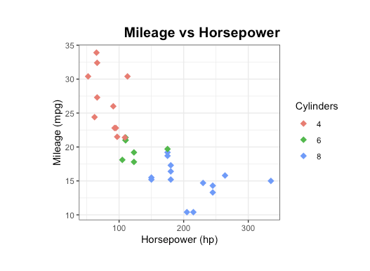
Let us start by creating a basic scatterplot of the mileage (mpg) of each car as a function of its horsepower (hp). In this case the data is our dataframe mtcars, and the aesthetics x and y will be defined as the names of the columns we wish to plot along each axis — hp and mpg. We can also set the color aesthetic to indicate the number of cylinders (cyl) in each car. One of the reasons ggplot2 is so user-friendly is because each graph property can be tacked on to the same line of code with a + sign. Since we want a scatterplot, the geometry will be defined using geom_point().

# basic scatterplot
g <- ggplot(data = mtcars, aes(x = hp, y = mpg, color=cyl))
g + geom_point()

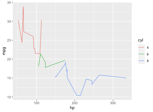
Excellent! The library automatically assigns the column names as axis labels, and uses the default theme and colors, but all of this can be modified to suit our tastes and to create pretty graphs. It is also important to note that we could have visualized the same data (less helpfully) as a line plot instead of a scatterplot, just by tweaking the geometry function.

# basic line plot
g + geom_line()

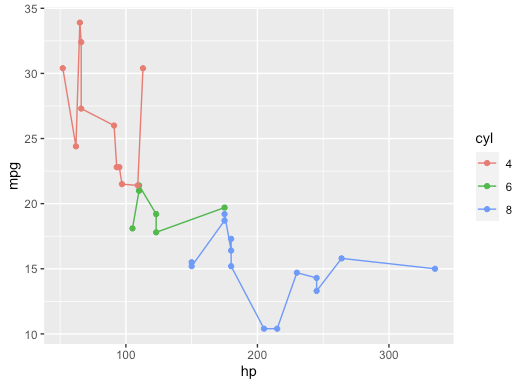
Well, this looks unpleasant. But wait, we can do so much more. We can also layer multiple geometries on the same graph to make more interesting plots.

# basic scatter+line plot
g + geom_line() + geom_point()

Additionally, we can tweak the geometry properties in each graph. Here is how we can transform the lines to dotted, and specify line widths and marker shape and size.

# change properties of geometry
g + geom_point(shape = "diamond", size = 3) +
  geom_line(color = "black", linetype = "dotted", size = .3) 

While our graph looks much neater now, using a line plot is actually pretty unhelpful for our dataset since each data point is a separate car. We will stick with a scatterplot for the rest of this tutorial. However, the above sort of graph would work great for time series data or other data that measures change in one variable.

Axis labels

One of the cardinal rules of good data visualization is to add axis labels to your graphs. While R automatically set the axis labels to be column headers, we can override this to make the axis labels more informative with just one extra function.

# change axis titles
g + geom_point(shape = "diamond", size = 3) +
  labs(x = "Horsepower (hp)", y = "Mileage (mpg)")

Title

This graph is in serious need of a title to provide a reader some idea of what they’re looking at. There are actually multiple ways to add a graph title here, but I find it easiest to use ggtitle().

# add title
g + geom_point(shape = "diamond", size = 3) +
  labs(x = "Horsepower (hp)", y = "Mileage (mpg)") +
  ggtitle("Mileage vs Horsepower") 

Alright, having a title is helpful, but I don’t love it’s placement on the graph. R automatically left-aligns the title, where it clashes with the y-axis. I would much rather have the title right-aligned, in a bigger font, and bolded. Here is how to do that.

# change position of title
g + geom_point(shape = "diamond", size = 3) +
  labs(x = "Horsepower (hp)", y = "Mileage (mpg)") +
  ggtitle("Mileage vs Horsepower")  +
  theme(plot.title = element_text(hjust = 1, size = 15, face = "bold"))

Theme

There are ways to manually change the background and gridlines of ggplot2 graphs using theme(), but an easy workaround is to use the built-in themes. Which theme you use depends greatly on the graph type and formatting guidelines, but I personally like a white background, faint gridlines, and a bounding box. One thing to note here though is that theme_bw() overrides theme() so the order of these two matters.

# add theme
g + geom_point(shape = "diamond", size = 3) +
  labs(x = "Horsepower (hp)", y = "Mileage (mpg)") +
  ggtitle("Mileage vs Horsepower") +
  theme_bw() +
  theme(plot.title = element_text(hjust = 1, size = 15, face = "bold"))

We can also use the theme() function to change the base font size and font family. Shown below is how to increase the base font size to 15 and change the base font family to Courier.

# use theme to change base font family and font size
g + geom_point(shape = "diamond", size = 3) +
  labs(x = "Horsepower (hp)", y = "Mileage (mpg)") +
  ggtitle("Mileage vs Horsepower")  +
  theme_bw(base_size = 15, base_family = "Courier") +
  theme(plot.title = element_text(hjust = 1, size = 15, face = "bold"))

Legend

It has been bothering me for the last seven paragraphs that my legend title still uses the column name. However, this is an easy fix. All I have to do is add a label to the color aesthetic in the labs() function.

# change legend title
g + geom_point(shape = "diamond", size = 3) +
  labs(x = "Horsepower (hp)", y = "Mileage (mpg)", color = "Cylinders") +
  ggtitle("Mileage vs Horsepower") +
  theme_bw() +
  theme(plot.title = element_text(hjust = 1, size = 15, face = "bold"))

We can also change the position of the legend. R automatically places legends on the right, and while I like having it to the right in this case, I could also place the legend at the bottom of the graph. This automatically changes the aspect ratio of the graph.

# change legend position
g + geom_point(shape = "diamond", size = 3) +
  labs(x = "Horsepower (hp)", y = "Mileage (mpg)", color = "Cylinders") +
  ggtitle("Mileage vs Horsepower") +
  theme_bw() +
  theme(plot.title = element_text(hjust = 1, size = 15, face = "bold")) +
  theme(legend.position = "bottom")

Margins

The theme() function is of endless use in ggplot2, and can be used to manually adjust the graph margins and add/remove white space padding. The order of arguments in margin() is counterclockwise — top, right, bottom, left (helpfully remembered by the pneumonic TRouBLe).

# add plot margins
g + geom_point(shape = "diamond", size = 3) +
  labs(x = "Horsepower (hp)", y = "Mileage (mpg)", color = "Cylinders") +
  ggtitle("Mileage vs Horsepower") +
  theme_bw() +
  theme(plot.title = element_text(hjust = 1, size = 15, face = "bold")) +
  theme(legend.position = "right") +
  theme(plot.margin = margin(t = 1, r = 1, b = 1, l = 2, unit = "cm"))

Conclusion

I have barely scratched the surface of what can be achieved using ggplot2 in this post. There are hundreds of excellent tutorials online that dive deeper into ggplot2, like this blog post by Cedric Scherer. I have yet to learn so much about this library and data visualization in general, but have hopefully made a solid case for using ggplot2 to create clean and aesthetically-pleasing data visualizations.

NetCDF Operators

This post is an introduction to Linux-based climate data and NetCDF operators (CDOs or NCOs) which allow you to perform various operations on netNDF files through the command line. I found these commands to be really nifty when I was working with pre-industrial control runs from a GCM. The output was being written on daily timestep, across 1200 years, and for the whole world, so it was absolutely essential that I cut the size of the files down as much as I could before transferring to my own computer.

The official documentation and installation instructions for NCO can be found here and CDO here, but if you’re working on a supercomputer, the libraries will already likely be installed. I will outline how I used some of these functions for my pre-industrial runs.

Concatenation

Some of the NCO commands have size limits of 40 GB, so it’s important to use the right order of operations when processing your files, which will be different depending on your ultimate goal. My goal was to ultimately get the 500-hpa geopotential height anomalies across the whole 1200 year period for specifically the Western US. Assuming you have a directory with all the NetCDF files, the first goal is to concatenate the data, since my run was broken into many smaller files. The easiest way to do this is with the following command which will take all the netcdf files in the directory (using the *) and merge them into a file called merged_file.nc:

cdo mergetime *.nc merged_file.nc

Return Individual Monthly Files

When calculating anomalies, you will need to determine a mean geopotential height value for each of the 12 months, and then calculate daily deviations with respect to these months to obtain daily deviations. You can do this with the following command:

cdo splitmon merged_file.nc zg500.mon

This command will return 12 files of the form zg500.mon$i.nc.

Return Monthly Means and Daily Anomalies

The next step is to calculate a monthly mean for each of these files. For example, for January use:

cdo timmean zg500.mon1.nc zg500.mean.mon1.nc

Return Anomalies

Now we subtract the means from each monthly file to return the daily anomalies for each month, which will be of the form: zg500.mean.mon${i}.anom.nc. If you want to combine the last two steps into one loop, you can use the code below:

for i in $(seq 1 12)
do
  cdo timmean zg500.mon${i}.nc zg500.mean.mon${i}.nc
  cdo sub zg500.mon${i}.nc zg500.mean.mon${i}.nc zg500.mean.mon${i}.anom.nc
done 

Cut Down to Geographical Area of Interest

Finally, we need to cut down the data just to the Western US. We use ncks (NetCDF Kitchen Sink) from NCO, which is probably the most versatile of all the functions (hence the name). This command is one that has the 40 GB limit, which is why I had to wait until I had monthly files before I could cut them down geographically. We must first specify the variable of interest using the -v flag. In my case, I only had one variable to extract, but you can also extract multiple in one command. Then denote the range of latitude and longitude using the -d flags. It is very important to include the periods at the end of each lat/lon (even if your bounds are integers) otherwise the command does not work.

for i in $(seq 1 12)
do
  ncks -v zg500 -d lon,180.,260. -d lat,30.,60. zg500.mean.mon${i}.cut.anom.nc -o zg500.mean.mon${i}.cut.anom.region.nc
done 

Ultimately, you will get 12 files of the form: zg500.mean.mon${i}.cut.anom.region.nc. And that’s it! You can concatenate the monthly files back together and try to resort the data back into the correct sequence according to time. I was unsuccessful at finding a quick way to do this, but it is possible. I found it much easier to work on this within R. I imported each of the 12 anomaly files, assigned a time vector, concatenated each monthly anomaly matrix into a larger matrix and then sorted according to date. If your files are small enough by the end of the process, this likely is the easiest way to take care of resorting. Enjoy!

Automate remote tasks with Paramiko

This is a short blogpost to demonstrate a the Paramiko Python package. Paramiko allows you to establish SSH, SCP or SFTP connections within Python scripts, which is handy when you’d like to automate some repetitive tasks with on remote server or cluster from your local machine or another cluster you’re running from.

It is often used for server management tasks, but for research applications you could consider situations where we have a large dataset stored at a remote location and are executing a script that needs to transfer some of that data depending on results or new information. Instead of manually establishing SSH or SFTP connections, those processes could be wrapped and automated within your existing Python script.

To begin a connection, all you need is a couple lines:

import paramiko

ssh_client = paramiko.SSHClient()
ssh_client.set_missing_host_key_policy(paramiko.AutoAddPolicy())
ssh_client.connect(hostname='remotehose',username='yourusername',password='yourpassword')

The first line creates a paramiko SSH client object. The second line tells paramiko what to do if the host is not a known host (i.e., whether this host should be trusted or not)—think of when you’re setting up an SSH connection for the first time and get the message:

The authenticity of host ‘name’ can’t be established. RSA key fingerprint is ‘gibberish’. Are you sure you want to continue connecting (yes/no)?

The third line is what makes the connection, the hostname, username and password are usually the only necessary things to define.

Once a connection is established, commands can be executed with exec_command(), which creates three objects:

stdin, stdout, stderr = ssh_client.exec_command("ls")

stdin is write-only file which can be used for commands requiring input, stdout contains the output of the command, and stderr contains any errors produced by the command—if there are no errors it will be empty.

To print out what’s returned by the command, use can use stdout.readlines(). To add inputs to stdin, you can do so by using the write() function:

stdin, stdout, stderr = ssh.exec_command(“sudo ls”)
stdin.write(‘password\n’)

Importantly: don’t forget to close your connection, especially if this is an automated script that opens many of them: ssh_client.close().

To transfer files, you need to establish an SFTP or an SCP connection, in a pretty much similar manner:

ftp_client=ssh_client.open_sftp()
ftp_client.get('/remote/path/to/file/filename','/local/path/to/file/filename')
ftp_client.close()

get() will transfer a file to a local directory, put(), used in the same way, will transfer a file to a remote directory.

More Terminal Schooling

You are probably asking yourself “and why do I need more terminal schooling?”. The short answer is: to not have to spend as much time as you do on the terminal, most of which spent (1) pushing arrow keys thousands of times per afternoon to move through a command or history of commands, (2) waiting for a command that takes forever to be done running before you can run anything else, (3) clicking all over the place on MobaXTerm and still feeling lost, (4) manually running the same command multiple times with different inputs, (5) typing the two-step verification token every time you want to change a “+” to a “-” on a file on a supercomputer, (6) waiting forever for a time-consuming run done in serial on a single core, and (7, 8, …) other useless and horribly frustrating chores. Below are some tricks to make your Linux work more efficient and reduce the time you spend on the terminal. From now on, I will use a “$” sign to indicate that what follows is a command typed in the terminal.

The tab autocomple is your best friend

When trying to do something with that file whose name is 5480458 characters long, be smart and don’t type the whole thing. Just type the first few letters and hit tab. If it doesn’t complete all the way it’s because there are multiple files whose names begin with the sequence of characters. In this case, hitting tab twice will return the names of all such files. The tab autocomplete works for commands as well.

Ctrl+r for search through previous commands

When on the terminal, hit ctrl+r to switch to reverse search mode. This works like a simple search function o a text document, but instead looking in your bash history file for commands you used over the last weeks or months. For example, if you hit ctrl+r and type sbatch it will fill the line with the last command you ran that contained the word sbatch. If you hit ctrl+r again, it will find the second last used command, and so on.

Vim basics to edit files on a system that requires two-step authentication

Vim is one the most useful things I have came across when it comes to working on supercomputers with two-step identity verification, in which case using MobaXTerm of VS Code requires typing a difference security code all the time. Instead of uploading a new version of a code file every time you want to make a simple change, just edit the file on the computer itself using Vim. To make simple edits on your files, there are very few commands you need to know.

To open a file with Vim from the terminal: $ vim <file name> or $ vim +10 <file name>, if you want to open the file and go straight to line 10.

Vim has two modes of operation: text-edit (for you to type whatever you want in the file) and command (replacement to clicking on file, edit, view, etc. on the top bar of notepad). When you open Vim, it will be in command mode.

To switch to text-edit mode, just hit either “a” or “i” (you should then see “– INSERT –” at the bottom of the screen). To return to command mode, hit escape (Esc). When in text-edit more, the keys “Home,” “End,” “Pg Up,” “Pg Dn,” “Backspace,” and “Delete” work just like on Notepad and MS Word.

When in command mode, save your file by typing :w + Enter, save and quite with :wq, and quit without saving with :q!. Commands for selecting, copying and pasting, finding and replacing, replacing just one character, deleting a line, and other more advanced tasks can be found here. There’s also a great cheatsheet for Vim here. Hint: once you learn some more five to ten commands, making complex edits on your file with Vim becomes blazingly fast.

Perform repetitive tasks on the terminal using one-line Bash for-loops.

Instead of manually typing a command for each operation you want to perform on a subset of files in a directory (“e.g., cp file<i>.csv directory300-400 for i from 300 to 399 , tar -xzvf myfile<i>.tar.gz, etc.), you can use a Bash for-loop if using the is not possible.

Consider a situation in which you have 10,000 files and want to move files number 200 to 299 to a certain directory. Using the wildcard “*” in this case wouldn’t be possible, as result_2<i>.csv would return result_2.csv, result_20.csv to result_29.csv, and result_2000.csv to result_2999.csv as well–sometimes you may be able to use Regex, but that’s another story. To move a subset of result files to a directory using a Bash for-loop, you can use the following syntax:

$ for i in {0..99}; do cp result_2$i results_200s/; done

Keep in mind that you can have multiple commands inside a for-loop by separating them with “;” and also nest for-loops.

Run a time-intensive command on the background with an “&” and keep doing your terminal work

Some commands may take a long time to run and render the terminal unusable until it’s complete. Instead of opening another instance of the terminal and login in again, you can send a command to the background by adding “&” at the end of it. For example, if you want to extract a tar file with dozens of thousands of files in it and keep doing your work as the files are extracted, just run:

$ tar -xzf my_large_file.tar.gz &

If you have a directory with several tar files and want to extract a few of them in parallel while doing your work, you can use the for-loop described above and add “&” to the end of the tar command inside the loop. BE CAREFUL, if your for-loop iterates over dozens or more files, you may end up with your terminal trying to run dozens or more tasks at once. I accidentally crashed the Cube once doing this.

Check what is currently running on the terminal using ps

To make sure you are not overloading the terminal by throwing too many processes at it, you can check what it is currently running by running the command ps. For example, if I run an program with MPI creating two processes and run ps before my program is done, it will return the following:

bernardoct@DESKTOP-J6145HK /mnt/c/Users/Bernardo/CLionProjects/WaterPaths
$ mpirun -n 2 ./triangleSimulation -I Tests/test_input_file_borg.wp &
[1] 6129     <-- this is the process ID
bernardoct@DESKTOP-J6145HK /mnt/c/Users/Bernardo/CLionProjects/WaterPaths
 $ ps
 PID TTY TIME CMD
 8 tty1 00:00:00 bash
 6129 tty1 00:00:00 mpirun    <-- notice the process ID 6129 again
 6134 tty1 00:00:00 triangleSimulat
 6135 tty1 00:00:00 triangleSimulat
 6136 tty1 00:00:00 ps

Check the output of a command running on the background

If you run a program on the background its output will not be printed on the screen. To know what’s happening with your program, send (to pipe) its output to a text file using the “>” symbol, which will be updated continuously as your program is running, and check it with cat <file name>, less +F<file name>, tail -n<file name>, or something similar. For example, if test_for_background.sh is a script that will print a number on the screen every one second, you could do the following (note the “> pipe.csv” in the first command):

bernardoct@DESKTOP-J6145HK /mnt/c/Users/Bernardo/CLionProjects/WaterPaths
 $ ./test_for_background.sh > pipe.csv &
 [1] 6191

bernardoct@DESKTOP-J6145HK /mnt/c/Users/Bernardo/CLionProjects/WaterPaths
 $ cat pipe.csv
 1
 2

bernardoct@DESKTOP-J6145HK /mnt/c/Users/Bernardo/CLionProjects/WaterPaths
 $ cat pipe.csv
 1
 2
 3

bernardoct@DESKTOP-J6145HK /mnt/c/Users/Bernardo/CLionProjects/WaterPaths
 $ tail -3 pipe.csv
 8
 9
 10

This is also extremely useful in situations when you want to run a command that takes long to run but whose outputs are normally displayed one time on the screen. For example, if you want to check the contents of a directory with thousands of files to search for a few specific files, you can pipe the output of ls to a file and send it to the background with ls > directory_contents.txt & and search the resulting text file for the file of interest.

System monitor: check core and memory usage with htop, or top if htop is not available

If ps does not provide enough information given your needs, such as if you’re trying to check if your multi-thread application is using the number of cores it should, you can try running htop instead. This will show on your screen something along the lines of the Performance view  of Windows’ Task Manager, but without the time plot. It will also show how much memory is being used, so that you do not accidentally shut down a node on an HPC system. If htop is not available, you can try top.

Running make in parallel with make -j for much shorter compiling time

If a C++ code is properly modularized, make can compile certain source code files in parallel. To do that, run make -j<number of cores> <rule in makefile>. For example, the following command would compile WaterPaths in parallel over four cores:

$ make -j4 gcc

For WaterPaths, make gcc takes 54s on the Cube, make -j4 gcc takes 15s, make -j8 gcc takes 9s, so the time and patience savings are real if you have to compile the code various times per day. To make your life simpler, you can add an alias to bash_aliases such as alias make='make -j4' (see below in section about .bash_aliases file). DO NOT USE MAKE -J ON NSF HPC SYSTEMS: it is against the rules. On the cube keep it to four cores or less not to disturb other users, but use all cores available if on the cloud or iterative section.

Check the size of files and directories using du -hs

The title above is quite self-explanatory. Running du -hs <file name> will tell you its size.

Check the data and time a file was created or last modified using the stat command

Also rather self-explanatory. Running stat <file name> is really useful if you cannot remember on which file you saved the output last time you ran your program.

Split large files into smaller chunks with the split command and put them back together with cat

This works for splitting a large text file into files with fewer lines, as well as for splitting large binary files (such as large tar files) so that you can, for example, upload them to GitHub or e-mail them to someone. To split a text file with 10,000 into ten files with 1,000 lines each, use:

 $ split -l 1000 myfile myfile_part

This will result in ten files called myfile_part00, myfile_part01, and so on with 1,000 lines each. Similarly, the command below would break a binary file into parts with 50 MB each:

 $ split -b 50m myfile myfile_part

To put all files back together in either case, run:

$ cat myfile_part* myfile

More information about the split command can be found in Joe’s post about it.

Checking your HPC submission history with `sacct`

Another quite sulf-explanatory tile. If you want to remember when you submitted something, such as to check if an output file resulted from this or that submission (see stat command), just run the command below in one line:

$ sacct -S 2019-09-18 -u bct52 --format=User,JobID,Jobname,start,end,elapsed,nnodes,nodelist,state

This will result in an output similar to the one below:

bct52 979 my_job 2019-09-10T21:48:30 2019-09-10T21:55:08 00:06:38 1 c0001 COMPLETED
bct52 980 skx_test_1 2019-09-11T01:44:08 2019-09-11T01:44:09 00:00:01 1 c0001 FAILED
bct52 981 skx_test_1 2019-09-11T01:44:33 2019-09-11T01:56:45 00:12:12 1 c0001 CANCELLED
bct52 1080 skx_test_4 2019-09-11T22:07:03 2019-09-11T22:08:39 00:01:36 4 c[0001-0004] COMPLETED
1080.0 orted 2019-09-11T22:08:38 2019-09-11T22:08:38 00:00:00 3 c[0002-0004] COMPLETED

Compare files with meld, fldiff, or diff

There are several programs to show the differences between text files. This is particularly useful when you want to see what the changes between different versions of the same file, normally a source code file. If you are on a computer running a Linux OS or have an X server like Xming installed, you can use meld and kdiff3 for pretty outputs on a nice GUI or fldiff to quickly handle a files with huge number of difference. Otherwise, diff will show you the differences in a cruder pure-terminal but still very much functional manner. The syntax for all of them is:

$ <command> <file1> <file2>

Except for diff, for which it is worth calling with the --color option:

$ diff --color <file1> <file2>

If cannot run a graphical user interface but is feeling fancy today, you can install the ydiff Python extension with (done just once):

$ python3 -m pip install --user ydiff 

and pipe diff’s output to it with the following:

$diff -u <file1> <file2> | python3 -m ydiff -s

This will show you the differences between two versions of a code file in a crystal clear, side by side, and colorized way.

Creating a .bashrc file for a terminal that’s easy to work with and good (or better) to look at

When we first login to several Linux systems the terminal is all black with white characters, in which it’s difficult find the commands you typed amidst all the output printed on the screen, and with limited autocomplete and history search. In short, it’s a real pain and you makes you long for Windows as much as for you long for your mother’s weekend dinner. There is, however, a way of making the terminal less of a pain to work with, which is by creating a file called .bashrc with the right contents in your home directory. Below is an example of a .bashrc file with the following features for you to just copy and paste in your home directory (e.g., /home/username/, or ~/ for short):

  • Colorize your username and show the directory you’re currently in, so that it’s easy to see when the output of a command ends and the next one begins–as in section “Checking the output of a command running on the background.”
  • Allow for a search function with the up and down arrow keys. This way, if you’re looking for all the times you typed a command starting with sbatch, you can just type “sba” and hit up arrow until you find the call you’re looking for.
  • A function that allows you to call extract and the compressed file will be extracted. No more need to tar with a bunch of options, unzip, unrar, etc. so long as you have all of them installed.
  • Colored man pages. This means that when you look for the documentation of a program using man, such as man cat to see all available options for the cat command, the output will be colorized.
  • A function called pretty_csv to let you see csv files in a convenient, organized and clean way from the terminal, without having to download it to your computer.
# .bashrc

# Source global definitions
if [ -f /etc/bashrc ]; then
. /etc/bashrc
fi

# Load aliases
if [ -f ~/.bash_aliases ]; then
. ~/.bash_aliases
fi

# Automatically added by module
shopt -s expand_aliases

if [ ! -z "$PS1" ]; then
PS1='\[\033[G\]\[\e]0;\w\a\]\n\[\e[1;32m\]\u@\h \[\e[33m\]\w\[\e[0m\]\n\$ '
bind '"\e[A":history-search-backward'
bind '"\e[B":history-search-forward'
fi

set show-all-if-ambiguous on
set completion-ignore-case on
export PATH=/usr/local/gcc-7.1/bin:$PATH
export LD_LIBRARY_PATH=/usr/local/gcc-7.1/lib64:$LD_LIBRARY_PATH

history -a
export DISPLAY=localhost:0.0

sshd_status=$(service ssh status)
if [[ $sshd_status = *"is not running"* ]]; then
sudo service ssh --full-restart
fi

HISTSIZE=-1
HISTFILESIZE=-1

extract () {
if [ -f $1 ] ; then
case $1 in
*.tar.bz2)   tar xvjf $1    ;;
*.tar.gz)    tar xvzf $1    ;;
*.bz2)       bunzip2 $1     ;;
*.rar)       unrar x $1       ;;
*.gz)        gunzip $1      ;;
*.tar)       tar xvf $1     ;;
*.tbz2)      tar xvjf $1    ;;
*.tgz)       tar xvzf $1    ;;
*.zip)       unzip $1       ;;
*.Z)         uncompress $1  ;;
*.7z)        7z x $1        ;;
*)           echo "don't know how to extract '$1'..." ;;
esac
else
echo "'$1' is not a valid file!"
fi
}

# Colored man pages
export LESS_TERMCAP_mb=$'\E[01;31m'
export LESS_TERMCAP_md=$'\E[01;31m'
export LESS_TERMCAP_me=$'\E[0m'
export LESS_TERMCAP_se=$'\E[0m'
export LESS_TERMCAP_so=$'\E[01;44;33m'
export LESS_TERMCAP_ue=$'\E[0m'
export LESS_TERMCAP_us=$'\E[01;32m'

# Combine multiline commands into one in history
shopt -s cmdhist

# Ignore duplicates, ls without options and builtin commands
HISTCONTROL=ignoredups
export HISTIGNORE="&:ls:[bf]g:exit"

pretty_csv () {
cat "$1" | column -t -s, | less -S
}

There are several .bashrc example files online with all sorts of functionalities. Believe me, a nice .bashrc will make your life A LOT BETTER. Just copy and paste the above into a text file called .bashrc and sent it to your home directory in your local or HPC system terminal.

Make the terminal far less user-friendly and less archane by setting up a .bash_aliases file

You should also have a .bash_aliases file to significantly reduce typing and colorizing the output of commands you often use for ease of navigation. Just copy all the below into a file called .bash_aliases and copy into your home directory (e.g., /home/username/, or ~/ for short). This way, every time you run the command between the word “alias” and the “=” sign, the command after the “=”sign will be run.

alias ls='ls --color=tty'
alias ll='ls -l --color=auto'
alias lh='ls -al --color=auto'
alias lt='ls -alt --color=auto'
alias uu='sudo apt-get update && sudo apt-get upgrade -y'
alias q='squeue -u '
alias qkill='scancel $(qselect -u bct52)'
alias csvd="awk -F, 'END {printf \"Number of Rows: %s\\nNumber of Columns: %s\\n\", NR, NF}'"
alias grep='grep --color=auto'                          #colorize grep output
alias gcc='gcc -fdiagnostics-color=always'                           #colorize gcc output
alias g++='g++ -fdiagnostics-color=always'                          #colorize g++ output
alias paper='cd /my/directory/with/my/beloved/paper/'
alias res='cd /my/directory/with/my/ok/results/'
alias diss='cd /my/directory/of/my/@#$%&/dissertation/'
alias aspell='aspell --lang=en --mode=tex check'
alias aspellall='find . -name "*.tex" -exec aspell --lang=en --mode=tex check "{}" \;'
alias make='make -j4'

Check for spelling mistakes in your Latex files using aspell

Command-line spell checker, you know what this is.

aspell --lang=en --mode=tex check'

To run aspell check on all the Latexfiles in a directory and its subdirectories, run:

find . -name "*.tex" -exec aspell --lang=en --mode=tex check "{}" \;

Easily share a directory on certain HPC systems with others working on the same project [Hint from Stampede 2]

Here’s a great way to set permissions recursively to share a directory named projdir with your research group:

$ lfs find projdir | xargs chmod g+rX

Using lfs is faster and less stressful on Lustre than a recursive chmod. The capital “X” assigns group execute permissions only to files and directories for which the owner has execute permissions.

Run find and replace in all files in a directory [Hint from Stampede 2]

Suppose you wish to remove all trailing blanks in your *.c and *.h files. You can use the find command with the sed command with in place editing and regular expressions to this. Starting in the current directory you can do:

$ find . -name *.[ch] -exec sed -i -e ‘s/ +$//’ {} \;

The find command locates all the *.c and *.h files in the current directory and below. The -exec option run the sed command replacing {} with the name of each file. The -i option tells sed to make the changes in place. The s/ +$// tells sed to replace one or blanks at the end of the line with nothing. The \; is required to let find know where the end of the text for the -exec option. Being an effective user of sed and find can make a great different in your productivity, so be sure to check Tina’s post about them.

Other post in this blog

Be sure to look at other posts in this blog, such as Jon Herman’s post about ssh, Bernardo’s post about other useful Linux commands organized by task to be performed, and Joe’s posts about grep (search inside multiple files) and cut.

Remote terminal environment using VS Code for Windows and Mac

On Windows machines, the application MobaXterm is a valuable tool for computing on virtual machines and working through SSH clients. David Gold’s blog post walks through the installation and use of this app, which works well in Windows environments.

Working remotely on my Mac laptop, I have been struggling to achieve the same workflow as in the office, with a Windows machine. Unfortunately, MobaXterm is not available for download on Mac OS. Looking for alternatives, I discovered that using VS Code with the “Remote – SSH” extension is a great replacement with significant advantages to MobaXterm, as it an SSH client interface and code editor in one.

A screenshot from my VS Code remote interface, with the graphical file browser on the left panel, the SSH server terminal on the bottom-right, and the VS Code editor on the top-right.

Here’s how you can set up a remote session on Mac (and Windows) using VS Code: 

  1. Install the VS Code application here. For installation help and a brief overview of the app, check out this video.
  2. With VS Code opened, go to View -> Extensions, and search “Remote – SSH.” Click on the extension and press the green “Install” button. You should see the message “This extension is enabled globally” appear. Check out this extension’s description below (I’ll run through the basics in this post).
  3. On the bottom left of your screen, there should be a small green box with two opposite pointing arrow heads. Click this.
The green box is the Remote – SSH extension.
  1. Choose the first pop-up option “Remote-SSH: Connect to host…” and then select “Add New SSH Host…”.
Click the first box and then the “Add New SSH Host” button to connect to your SSH client.
  1. Here, enter your remote SSH username@serverid (here at Cornell, this would be yournetid@thecube.cac.cornell.edu to connect to our remote computing cluster, the Cube).
  2. In the same pop-up window, click the remote server that you just added. A new window will open and prompt you to enter your password for the server.
  3. Now, you in are in your remote SSH environment. Click “Open folder…” and select “OK” to see your remote directory on the left. You can navigate through these files in your remote machine the same way as MobaXterm. Click View -> Terminal to see your SSH command line on the bottom of the screen (here’s where you can actually run the programs on your cluster).

Now using VS Code, you can install other extensions to aid in code editing in different languages (here’s an article with a few good ones for various uses). This environment has the same functionality as MobaXterm, without having to switch applications for editing code. Run your cluster programs in the terminal window and edit the code in the main VS Code editor!

Parallelization of C/C++ and Python on Clusters

There are multiple ways of parallelizing C/C++ and Python codes to be used on clusters. The quick and dirty way, which often gets the job done, is to parallelize the code with MPI and launch one process per core across multiple nodes. Though easy to implement, this strategy may result in a fair waste of results because:

  • With too many processes on one node, inefficient use of memory may make the code memory bottle-necked, meaning that a lot of time will be spent accessing memory and the cores will be sitting twiddling their thumbs.
  • If you have a 48-core node with 192 GB of memory (as the Skylake nodes on Stampede 2) and your code uses 10 GB of RAM per process, you will not be able to have more than 19 out of 48 cores working at the same time because more than that would exceed the node’s memory, which would crash the node, which would get you kicked out of the cluster for a while without a warning — if you do not know how much RAM your code requires, you should look into the Remora tool.

If you are working on big runs on systems that charge per usage time or if you are creating a code you will have to run multiple times, it may be worth looking into more clever parallelization strategies. Some of the techniques described in the next subsections will also make your code two to four times faster on your desktop/laptop and are rather straight-forward to implement. Most of the code in this blog post can be freely downloaded from this repository. Lastly, if the #include statements in the examples below are not displayed as followed by a library between “<>”, please refer to the mentioned online repository.

Hybrid Parallelization in C/C++

The word hybrid refers in this context to a mixed use of shared and distributed memory parallelization techniques. In distributed parallelization techniques, such as the Message Passing Interface (MPI), each process has its own dedicated chunk of memory within a RAM chip. This means that each process will have its own copy of the input data (repeated across processes), variables within the program, etc. Conversely, shared memory parallelization techniques such as OpenMP allow all threads (parallel unit of computation) to access the same block of memory, which can make a mess in your code with variables being changed seemingly out of nowhere by various parallel runs, but which lessens the amount of RAM needed and in some cases allow for more efficient memory utilization.

If running the Borg Master-Slave multiobjective evolutionary optimization algorithm (Borg MS) with hybrid parallelization, Borg MS will have each function evaluation performed by one MPI process, which could run in parallel with OpenMP (if your model is setup for that) across the cores designated for that process. As soon as a function evaluation is complete, the slave MPI process in charge of it will submit the results back to Borg MS’s master process and be given another set of decision variables to work on. The figure below is a schematic drawing of such hybrid parallelization scheme:

BorgHybridParallelization.png

OpenMP

Parallelizing a for-loop in C or C++ in which each iteration is independent — such as in Monte Carlo simulations — is straight-forward:

#include
#include "path/to/my_model.h"

int main(int argc, char *argv[])
{
    int n_monte_carlo_simulations = omp_get_num_threads(); // One model run per core.
    vector system_inputs = ;
    vector results(n_monte_carlo_simulations, 0);
#pragma omp parallel for
    for (int i = 0; i < n_monte_carlo_simulations; ++i)
    {
        results[i] = RunMonteCarloSimulation(system_inputs[i]);
    }
}

The only caveat is that you have to be sure that the independent simulations are not writing over each other. For example, if by mistake you had written results[0] instead of results[i], the final value on results[0] would be that of whichever thread (parallel simulation) finished last, while the rest of the vector would be of zeros. It is important to notice here that the vector system_inputs is read only once by the parallel code and all n_monte_carlo_simulations threads would have access to it in memory.

Though this example is not rocket science, there is a lot more to OpenMP that can be found here and here.

MPI

MPI stands for Message Passing Interface. It creates processes which pass messages (information packages) to each other. The most basic MPI code is one that creates independent processes — each with its own allocated chunk of memory that cannot be accessed by any other process — and just has them running independently in parallel without communicating with each other. This is great to distribute Monte Carlo runs across various nodes, although it may lead to the limitations mentioned in the beginning of this post. Below is an example of a very basic MPI code to run Monte Carlo simulations in parallel:

#include
#include "path/to/my_model.h"

int main(int argc, char *argv[])
{
    MPI_Init(NULL, NULL);

    int world_rank;
    MPI_Comm_rank(MPI_COMM_WORLD, &world_rank);

    vector system_inputs = ;
    RunMonteCarloSimulation(system_inputs[world_rank]);

    MPI_Finalize();
    return 0;
}

I will not cover in this post how to pass the output of the RunMonteCarloSimulation function back to a results vector, as in the previous example, because details of MPI is outside the scope of this post — a good MPI tutorial can be found here and great examples, including ones for Monte Carlo runs, can be found here. To run this code, you would have to compile it with mpicc mpi_demo.c -o MPIDemo and call it with the mpirun or mpiexec commands, which should be followed by the -n flag to specify the number of processes to be created, or mpirun -n 4 ./MPIDemo. The code above would run as many MonteCarlo simulations as there are processes (four processes if -n 4 was used), each with a rank (here a type of ID), and can be spread across as many nodes as you can get on a cluster. Each process of the code above would run on a core, which may result in the memory and/or processing limitations listed in the beginning of this post.

Mixing OpenMP and MPI

The ideal situation for most cases is when you use MPI to distribute processes across nodes and OpenMP to make sure that as many cores within a node as it makes sense to use are being used. To do this, you can use the structure of the code below.

#include
#include
#include
#include "path/to/my_model.cpp"

int main(int argc, char *argv[])
{
    MPI_Init(NULL, NULL);

    int world_rank;
    MPI_Comm_rank(MPI_COMM_WORLD, &world_rank);

    int n_cores = omp_get_num_threads(); // get number of cores available for MPI process.
    vector system_inputs = ;
    vector results(n_cores , 0);
#pragma omp parallel for
    for (int i = 0; i < n_cores ; ++i)
    {
        // printf("C hybrid. Process-thread: %s-%d\n", world_rank, omp_get_thread_num());
        results[i] = RunMonteCarloSimulation(system_inputs[i]);
    }

    MPI_Finalize();
    return 0;

}

If you comment lines 4 and 20 and uncomment line 19, compile the code with mpicc hybrid.c -o Hybrid -fopenmp, set the number of threads in the terminal to eight by running set OMP_NUM_THREADS=8, and call the resulting executable with the command mpirun -n 4 ./Hybrid, the executable will spawn four processes, each of which spawning eight threads and printing the following output:

C hybrid. Process-thread: 0-0
C hybrid. Process-thread: 0-1
C hybrid. Process-thread: 0-4
C hybrid. Process-thread: 0-5
C hybrid. Process-thread: 0-7
C hybrid. Process-thread: 0-6
C hybrid. Process-thread: 0-2
C hybrid. Process-thread: 0-3
C hybrid. Process-thread: 1-6
C hybrid. Process-thread: 1-0
C hybrid. Process-thread: 1-1
C hybrid. Process-thread: 1-3
C hybrid. Process-thread: 1-5
C hybrid. Process-thread: 1-4
C hybrid. Process-thread: 1-7
C hybrid. Process-thread: 1-2
C hybrid. Process-thread: 2-6
C hybrid. Process-thread: 2-0
C hybrid. Process-thread: 2-3
C hybrid. Process-thread: 2-7
C hybrid. Process-thread: 2-2
C hybrid. Process-thread: 2-4
C hybrid. Process-thread: 2-5
C hybrid. Process-thread: 2-1
C hybrid. Process-thread: 3-0
C hybrid. Process-thread: 3-1
C hybrid. Process-thread: 3-3
C hybrid. Process-thread: 3-4
C hybrid. Process-thread: 3-6
C hybrid. Process-thread: 3-7
C hybrid. Process-thread: 3-2
C hybrid. Process-thread: 3-5

The code above can be used to have one process per node (and therefore one copy of system_inputs per node) using as many threads as there are cores in that node — depending on the number of cores, it is sometimes more efficient to have two or three MPI processes per node, each using half or a third of the cores in that node. Below is a PBS job submission script that can be used to generate the output above — job submission scripts for Slurm to be used on Stampede 2 can be found here.

#!/bin/bash
#PBS -N test_hybrid
#PBS -l nodes=2:ppn=16
#PBS -l walltime=:00:30
#PBS -o ./output/hybrid_c.out
#PBS -e ./error/hybrid_c.err
module load openmpi-1.10.7-gnu-x86_64
export OMP_NUM_THREADS=8

set -x
cd "$PBS_O_WORKDIR"

# Construct a copy of the hostfile with only 16 entries per node.
# MPI can use this to run 16 tasks on each node.
export TASKS_PER_NODE=2
uniq "$PBS_NODEFILE"|awk -v TASKS_PER_NODE="$TASKS_PER_NODE" '{for(i=0;i nodefile

#cat nodefile
mpiexec --hostfile nodefile -n 4 -x OMP_NUM_THREADS ./Hybrid

Parallelizing Python on a Cluster

Python was not designed with shared-memory parallelization in mind, so its native parallelization library, the Multiprocessing library, does distributed-memory parallelization instead of shared. The issue with the Multiprocessing library is that it does not work across nodes, so you still need something like MPI. Here, we will use MPI4Py.

The code below parallelizes the function call across cores within the same node — please refer to this blog post for details about and other ways to use the Multiprocessing library.

from multiprocessing import Process, cpu_count

def do_something_useful(rank, shared_process_number):
    # Do something useful here.
    print 'Python hybrid, MPI_Process-local_process (not quite a thread): {}-{}'.format(rank, shared_process_number)

# Create node-local processes
shared_processes = []
#for i in range(cpu_count()):
for i in range(8):
    p = Process(target=do_something_useful, args=(i,))
    shared_processes.append(p)

# Start processes
for sp in shared_processes:
    sp.start()

# Wait for all processes to finish
for sp in shared_processes:
    sp.join()

By adding MPI4Py to the code above, following the same logic of the C/C++ example, we get the following result:

from mpi4py import MPI
from multiprocessing import Process, cpu_count

def do_something_useful(rank, shared_process_number):
    # Do something useful here.
    print 'Python hybrid, MPI_Process-local_process (not quite a thread): {}-{}'.format(rank, shared_process_number)

comm = MPI.COMM_WORLD
rank = comm.Get_rank()

print 'Calling Python multiprocessing process from Python MPI rank {}'.format(rank)

# Create shared-ish processes
shared_processes = []
#for i in range(cpu_count()):
for i in range(8):
    p = Process(target=do_something_useful, args=(rank, i))
    shared_processes.append(p)

# Start processes
for sp in shared_processes:
    sp.start()

# Wait for all processes to finish
for sp in shared_processes:
    sp.join()

comm.Barrier()

Calling the code above with mpirun -n 4 python hybrid_pure_python.py will first result in four MPI processes being spawned with ranks 1 through 4, each spawning eight local processes. The output should look similar to the one below:

Calling Python multiprocessing process from Python MPI rank 0
Calling Python multiprocessing process from Python MPI rank 1
Python hybrid, MPI_Process-local_process (not quite a thread): 1-0
Python hybrid, MPI_Process-local_process (not quite a thread): 0-0
Python hybrid, MPI_Process-local_process (not quite a thread): 1-1
Python hybrid, MPI_Process-local_process (not quite a thread): 0-1
Python hybrid, MPI_Process-local_process (not quite a thread): 1-2
Python hybrid, MPI_Process-local_process (not quite a thread): 0-2
Python hybrid, MPI_Process-local_process (not quite a thread): 0-3
Python hybrid, MPI_Process-local_process (not quite a thread): 1-3
Calling Python multiprocessing process from Python MPI rank 2
Calling Python multiprocessing process from Python MPI rank 3
Python hybrid, MPI_Process-local_process (not quite a thread): 1-4
Python hybrid, MPI_Process-local_process (not quite a thread): 0-4
Python hybrid, MPI_Process-local_process (not quite a thread): 0-5
Python hybrid, MPI_Process-local_process (not quite a thread): 1-5
Python hybrid, MPI_Process-local_process (not quite a thread): 1-6
Python hybrid, MPI_Process-local_process (not quite a thread): 0-6
Python hybrid, MPI_Process-local_process (not quite a thread): 1-7
Python hybrid, MPI_Process-local_process (not quite a thread): 0-7
Python hybrid, MPI_Process-local_process (not quite a thread): 2-0
Python hybrid, MPI_Process-local_process (not quite a thread): 3-0
Python hybrid, MPI_Process-local_process (not quite a thread): 3-1
Python hybrid, MPI_Process-local_process (not quite a thread): 2-1
Python hybrid, MPI_Process-local_process (not quite a thread): 3-2
Python hybrid, MPI_Process-local_process (not quite a thread): 2-2
Python hybrid, MPI_Process-local_process (not quite a thread): 3-3
Python hybrid, MPI_Process-local_process (not quite a thread): 2-3
Python hybrid, MPI_Process-local_process (not quite a thread): 3-4
Python hybrid, MPI_Process-local_process (not quite a thread): 2-4
Python hybrid, MPI_Process-local_process (not quite a thread): 2-5
Python hybrid, MPI_Process-local_process (not quite a thread): 3-5
Python hybrid, MPI_Process-local_process (not quite a thread): 3-6
Python hybrid, MPI_Process-local_process (not quite a thread): 3-7
Python hybrid, MPI_Process-local_process (not quite a thread): 2-6
Python hybrid, MPI_Process-local_process (not quite a thread): 2-7

Below is a PBS submission script that can be used with the code above:

#!/bin/bash
#PBS -N test_hybrid
#PBS -l nodes=2:ppn=16
#PBS -l walltime=00:01:00
#PBS -o ./output/hybrid_python.out
#PBS -e ./error/hybrid_python.err
module load python-2.7.5
export OMP_NUM_THREADS=8

set -x
cd "$PBS_O_WORKDIR"

# Construct a copy of the hostfile with only 16 entries per node.
# MPI can use this to run 16 tasks on each node.
export TASKS_PER_NODE=2
uniq "$PBS_NODEFILE"|awk -v TASKS_PER_NODE="$TASKS_PER_NODE" '{for(i=0;i nodefile

#cat nodefile
mpiexec --hostfile nodefile -n 4 -x OMP_NUM_THREADS python hybrid_pure_python.py

Parallelizing Monte Carlo Runs of C/C++ (or anything else) with Python

Very often we have to run the same model dozens to thousands of times for Monte-Carlo-style analyses. One option is to go on a cluster and submit dozens to thousand of jobs, but this becomes a mess for the scheduler to manage and cluster managers tend to not be very fond of such approach. A cleaner way of performing Monte Carlo runs in parallel is to write a code in Python or other language that spawns MPI processes which then call the model to be run. This can be done in Python with the subprocess library, as in the example below:

from mpi4py import MPI
import subprocess

comm = MPI.COMM_WORLD
rank = comm.Get_rank()

print 'Calling OpenmpTest from Python MPI rank {}'.format(rank)
function_call = ['./OpenmpTest', '{}'.format(rank)]
subprocess.call(function_call)

comm.Barrier()

Here, OpenmpTest is an executable compiled from the C-OpenMP code below:

#include
#include 

int main(int argc, char *argv[])
{
#pragma omp parallel for
    for (int i = 0; i < omp_get_num_threads(); ++i)
    {
        printf("C OpenMP. Process-thread: %s-%d\n", argv[1], i);
    }
    return 0;
}

Submitting the code above with following PBS job submission script should result in the output below.

#!/bin/bash
#PBS -N test_hybrid
#PBS -l nodes=2:ppn=16
#PBS -l walltime=00:01:00
#PBS -o ./output/hybrid_python_c.out
#PBS -e ./error/hybrid_python_c.err
module load python-2.7.5
export OMP_NUM_THREADS=8

set -x
cd "$PBS_O_WORKDIR"

# Construct a copy of the hostfile with only 16 entries per node.
# MPI can use this to run 16 tasks on each node.
export TASKS_PER_NODE=2
uniq "$PBS_NODEFILE"|awk -v TASKS_PER_NODE="$TASKS_PER_NODE" '{for(i=0;i nodefile

#cat nodefile
mpiexec –hostfile nodefile -n 4 -x OMP_NUM_THREADS python hybrid_calls_c.py

Output:

Calling OpenmpTest from Python MPI rank 0
Calling OpenmpTest from Python MPI rank 1
Calling OpenmpTest from Python MPI rank 2
Calling OpenmpTest from Python MPI rank 3
C OpenMP. Process-thread: 0-7
C OpenMP. Process-thread: 0-5
C OpenMP. Process-thread: 0-0
C OpenMP. Process-thread: 0-2
C OpenMP. Process-thread: 0-4
C OpenMP. Process-thread: 0-1
C OpenMP. Process-thread: 0-3
C OpenMP. Process-thread: 0-6
C OpenMP. Process-thread: 1-1
C OpenMP. Process-thread: 1-2
C OpenMP. Process-thread: 1-6
C OpenMP. Process-thread: 1-4
C OpenMP. Process-thread: 1-5
C OpenMP. Process-thread: 1-0
C OpenMP. Process-thread: 1-3
C OpenMP. Process-thread: 1-7
C OpenMP. Process-thread: 2-3
C OpenMP. Process-thread: 2-7
C OpenMP. Process-thread: 2-0
C OpenMP. Process-thread: 2-4
C OpenMP. Process-thread: 2-6
C OpenMP. Process-thread: 2-5
C OpenMP. Process-thread: 2-1
C OpenMP. Process-thread: 2-2
C OpenMP. Process-thread: 3-5
C OpenMP. Process-thread: 3-1
C OpenMP. Process-thread: 3-4
C OpenMP. Process-thread: 3-2
C OpenMP. Process-thread: 3-7
C OpenMP. Process-thread: 3-3
C OpenMP. Process-thread: 3-0
C OpenMP. Process-thread: 3-6

End of the Story

As highlighted in the examples above (all of which can be download from here), creating parallel code is not rocket science and requires very few lines of code. The OpenMP and Multiprocessing parallelization tricks can save hours if you have to run a model several times on your personal computer, and paired with MPI these tricks can save you from hours to days in time and thousands of node-hours on clusters. I hope you make good use of it.