Introducing OpenMORDM

In this blog post, I will introduce a new open source library called OpenMORDM.  I will begin by defining MORDM (Multi-Objective Robust Decision Making), provide instructions for installing the software, and conclude with a case study.

What is MORDM?

Robust Decision Making (RDM) is an analytic framework developed by Robert Lempert and his collaborators at RAND Corporation that helps identify potential robust strategies for a particular problem, characterize the vulnerabilities of such strategies, and evaluate trade-offs among them [Lempert et al. (2006)]. Multiobjective Robust Decision Making (MORDM) is an extension of RDM to explicitly include the use of multiobjective optimization to discover robust strategies and explore the tradeoffs among multiple competing performance objectives [Kasprzyk et al. (2013)]. We encourage users to read these two articles to gain insight into these methods.

Lempert, R. J., D. G. Groves, S. W. Popper, and S. C. Bankes (2006). A General, Analytic Method for Generating Robust Strategies and Narrative Scenarios. Management Science, 52(4):514-528.

Kasprzyk, J. R., S. Nataraj, P. M. Reed, and R. J. Lempert (2013). Many objective robust decision making for complex environmental systems undergoing change. Environmental Modelling & Software, 42:55-71.

Installing OpenMORDM

OpenMORDM is an open source implementation of MORDM written in the R programming language.  Its source code is freely available at https://github.com/OpenMORDM/OpenMORDM.  Installation instructions are available for Windows, Linux, and Mac OS X.

Python users may also find the EMA Workbench useful.  The EMA Workbench is primarily designed for Exploratory Modeling & Analysis, but it shares many common components with OpenMORDM.

Case Study

It is perhaps best to introduce MORDM with an example.  We will use the Lake Problem, taken from the recently published paper:

Hadka, D., Herman, J., Reed, P.M., Keller, K. An Open Source Framework for Many-Objective Robust Decision Making. Environmental Modelling & Software, 74:114-129, 2015. DOI:10.1016/j.envsoft.2015.07.014.

An online version of this paper can be found here.

The Lake Problem models a hypothetical town situated near a lake. The lake provides tourism and recreation activities for the town, and thus the town’s inhabitants wish to maintain the quality of the lake. However, industrial activities and farming release pollutants into the lake. The goal of this exercise is to determine an acceptable level of pollution that can be released without polluting the lake. We will have to balance the desire for increased economic activity (which increases pollution) with the aversion to polluting the lake. A diagram of this system is shown below.

This system is driven by five parameters. mean and stdev control the amount of naturally-occurring pollution that enters the lake. This type of pollution can not be controlled. b and q control how quickly the lake can remove pollution through various natural processes. delta specifies the discount rate for valuing the economic benefit in future years.

Defining the Model in R

The R model for the Lake Problem is shown below. The argument decisions will reflect the level of allowed pollution. decisions will be a vector with 100 values, specifying the allowed pollution for each year in the 100 year simulation. The remaining arguments will remain fixed for this exercise.

lake.eval <- function(decisions, samples=100, days=100, b=0.42, q=2, mean=0.02,
                      stdev=0.001, delta=0.98, alpha=0.4, beta=0.08,
                      reliability.threshold=0.9, inertia.threshold=-0.02) {
    pcrit <- uniroot(function(y) y^q/(1+y^q) - b*y, c(0.01, 1.5))$root
    X <- rep(0, days)
    objs <- rep(0, 4)

    for (i in 1:samples) {
        X[1] <- 0
        natural.pollution <- rlnorm(days,
                                    log(mean^2/sqrt(stdev^2 + mean^2)),
                                    sqrt(log(1+stdev^2/mean^2)))

        for (t in 2:days) {
            X[t] <- (1-b)*X[t-1] + X[t-1]^q/(1+X[t-1]^q) + decisions[t] + natural.pollution[t]
        }

        objs[1] <- objs[1] + max(X) / samples
        objs[4] <- objs[4] - sum(X < pcrit) / (samples*days)
    }

    objs[2] <- -sum(alpha*decisions*delta^(1:days))
    objs[3] <- -sum(diff(decisions) > inertia.threshold) / (days-1)

    list(objectives=objs, constraints=max(reliability.threshold+objs[4], 0))
}

The Lake Problem has four objectives and one constraint. The four objectives measure the amount of pollution (phosphorus) in the lake, the economic benefit gained from polluting the lake, a restriction on how significant the pollution control strategy can change from year-to-year (inertia), and the probability that the lake becomes irreversibly polluted (reliability). The constraint requires that that lake must remain unpolluted for at least 90% of the time periods in each simulation.

The goal of this exercise is to find the optimal set of decisions that will minimize the pollution in the lake, maximize economic benefit, minimize the need for policy changes (inertia), and maximize the reliability. The optimal decisions depends on the system properties, primarily b, q, mean, stdev, and delta. In real-world scenarios, the values for these properties might not be known. In this case, we have estimated what the value should be. However, since we are not 100% certain that our estimates are correct, we say these parameters have well-characterized uncertainty. Later, we will discuss how to handle situations where the parameters or their distributions are not well-defined or cannot be reliably estimated, called “deep uncertainty”.

Connecting the Model to OpenMORDM

Models are connected to OpenMORDM using the define.problem function. To see the documentation for this function, run ?define.problem within R. The first four arguments to define.problem is the function (either an R function or the command line to invoke the executable) and the number of inputs, outputs, and constraints, respectively.

library(OpenMORDM)

nvars <- 100
nobjs <- 4
nconstrs <- 1

problem <- define.problem(lake.eval, nvars, nobjs, nconstrs,
    bounds=matrix(rep(range(0, 0.1), nvars), nrow=2),
    names=c("Phosphorus in Lake", "Economic Benefit", "Inertia", "Reliability"),
    maximize=c("Economic Benefit", "Inertia", "Reliability"),
    epsilons=c(0.0001,0.0001,0.000001,0.000001))

bounds specifies the lower and upper bounds of the decisions (or model inputs). In this exercise, we have 100 decisions (one for each year) ranging from [0, 0.1]. names provides a list of names for the objectives. These names are used later when generating plots. maximize indicates which objectives are maximized. By default, OpenMORDM assumes all objectives are minimized unless specified by this argument. epsilons specifies the resolution of solutions for each objective. OpenMORDM automatically ignores solutions whose differences are less than the specified resolution. This avoids enumerating a potentially infinite number of solutions. Larger epsilons will result in fewer solutions, and vice versa.

Optimizing the Model

Before we begin, first ensure the Borg MOEA is installed on your computer by following the steps to install the Borg MOEA. Once setup, we can optimize the model to discover the best pollution control strategy for the Lake Problem given our well-characterized uncertainties:

data <- borg.optimize(problem, 100000)

It will take several minutes for the optimization to run. Once finished, we can generate a 3D plot and a parallel coordinates plot of the best solutions:

palette <- colorRampPalette(c("green", "yellow", "red"))(100)
mordm.plot(data, color="Reliability", palette=palette)
mordm.plot.parallel(line.width=3)

We are defining a custom color palette so that green solutions have good reliability and red solutions have poor reliability. The resulting figures will appear similar to:

You’ll note that there are many “best” solutions. Since the model has multiple performance objectives, we typically find solutions that are better in some objectives and worse in others. However, no solution is clearly best (e.g., better in all objectives). For this reason, this is often referred to as the “Pareto set” since it contains the Pareto efficient solutions.

Adding Deep Uncertainties

In the previous section, we optimized the Lake Problem under well-characterized uncertainty. That is to say we were able to make an educated guess or reasonably estimate the model parameters. In many situations, estimating the model parameters is not possible. This is called “deep uncertainty”.

In MORDM, we can model deep uncertainty by defining additional distributions on the model parameters. For the Lake Problem, we identify five deeply-uncertain variables: b, q, mean, stdev, and delta. b and q correspond to the removal of pollution from the lake due to natural processes, mean and sigma control the inflow of naturally-occurring pollution into the lake, and delta is our discounting factor.

param_names <- c("b", "q", "mean", "stdev", "delta")
baseline_SOW <- c(0.42, 2, 0.02, 0.0017, 0.98)

When we optimized the Lake Problem under well-characterized uncertainty, we used baseline values for these five parameters. If it turns out our baseline values were incorrect in the future, then our predictions based on the model will be incorrect. For the Lake Problem, this means we may end up over-polluting the lake and rendering it inhospitable. We would like to provide better advice, and therefore want to determine how robust our pollution control strategy is to such uncertainties. To do so, we will define lower and upper bounds based on what is feasible and generate 1000 hypothetical futures, called states of the world (SOWs), within these new bounds. These hypothetical states of the world may not actually occur in reality, but we can attempt to find pollution control strategies that work well across all of these states of the world. If we can do so, then our policy will be robust regardless of the future conditions.

nsamples <- 1000

SOWS <- sample.lhs(nsamples,
                   b=c(0.1, 0.45),
                   q=c(2, 4.5),
                   mean=c(0.01, 0.05),
                   stdev=c(0.001, 0.005),
                   delta=c(0.93, 0.99))

Next, we define many models, one for each of the sampled SOWs. Within each model, the parameters to our R function, lake.eval, are being replaced with the sampled values for each SOW.

models <- create.uncertainty.models(problem, factors)

Note: these two methods, sample.lhs and create.uncertainty.models, only work for models written in R. If your model is not an R function, refer to the example in the supplemental materials.

Next, we take our Pareto set of solutions we generated in the previous section and see how well they perform in the future SOWs. The following command takes each solution in the Pareto set and runs it against each SOW:

uncertainty.samples <- mordm.sample.uncertainties(data, nsamples, models)

When we run each solution against the SOW, we expect that the performance objectives will change given the new model parameters. There are different ways to measure how significantly a solution is affected by these changes. One such way, which we call “Regret Type 1” is to measure the deviation in performance within each state of the world against the performance of the baseline solution (under well-characterized uncertainty). Larger deviations indicate we may regret our policy choice if it performs differently than what we expect. Another measure, called “Satisfying Type 1”, looks at the percentage of SOWs where some criteria is satisfied. This criteria can be anything, and for this exercise, we want to ensure the reliability is > 75% (the lake becomes overpolluted in fewer than 15% of the simulations) and our economic benefit is > 0.2. We encode these criteria with the function function(x) sum(abs(x$constrs)) == 0 && x$objs["Economic Benefit"]>0.1. We can compute these robustness measures as follows:

robustness <- mordm.evaluate.uncertainties(uncertainty.samples,
    function(x) sum(abs(x$constrs)) == 0 && x$objs[2]>0.1,
    SOWS,
    baseline_SOW)

mordm.plot(data, color=robustness[,"Regret Type I"], palette=palette)
mordm.plot(data, color=robustness[,"Satisficing Type I"], palette=palette)

Like before, the color green indicates better robustness to the deep uncertainties. You may notice that the two robustness measures produce different results. How we define robustness can produce dramatically different results, and we must always consider the consequences of our experimental design. However, OpenMORDM lets us compare different robustness measures so we can become better informed.

Identifying Vulnerabilities

Suppose we have identified one solution of particular interest. In the 3D plots generated by mordm.plot, you can click any point with the middle-mouse button to see its index number. Lets say we are interested in solution #17

selected.point <- uncertainty.samples[[17]]

Even though we identified that this design is robust to deep uncertainty, it still may fail in some of the states of the world. We now want to determine what caused those failures. There are two methods we will discuss for this task: PRIM and CART.

Patient Rule Induction Method (PRIM)

The Patient Rule Induction Method (PRIM) is a data mining technique (sometimes referred to as “bump hunting”) for finding regions in high-dimensional space where a response variable has a predominantly high (or low) value. PRIM works by iteratively “peeling”, or removing, a small portion of the samples with the lowest (or highest) response value. For this example, we want to determine what causes poor reliability (e.g., a high likelihood of overpolluting the lake). Therefore, we will use PRIM to identify the region(s) where the mean reliability is minimal.

analyze.prim(SOWS, selected.point$objs[,"Reliability"], threshold.type=-1)

The resulting PRIM box is shown below:

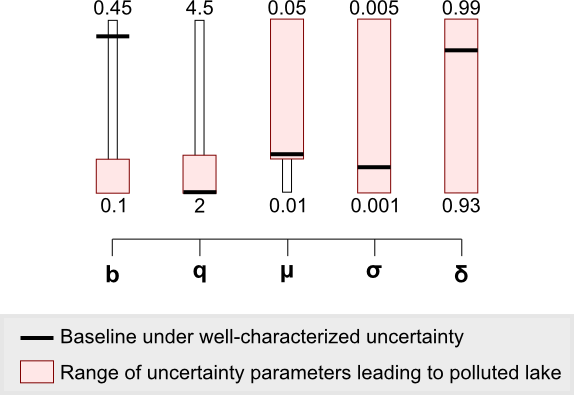Each uncertainty parameter is shown as a vertical bar and the red region indicates where poor reliability is observed. We want to avoid parameters falling within the red regions. In this exercise, since the parameters represent naturally-occurring factors we can not control, these red regions instead act as monitoring signposts. If in the future we determine the lake’s true parameters fall within the red regions, then we know there is a higher likelihood that the lake will become polluted given the implemented pollution control policy. If this were to occur, we would need to become proactive to avoid polluting the lake.

Classification and Regression Trees (CART)

Classification and Regression Trees (CART) recursively partition the samples within a dataset. When using CART for classification, the dataset is partitioned to predict the sample category. Here, we will assign two categories, Unpolluted and Polluted, and use CART to determine the rules partitioning these two categories.

analyze.cart(SOWS, ifelse(selected.point$objs[,"Reliability"]<1,
    "Polluted", "Unpolluted"))

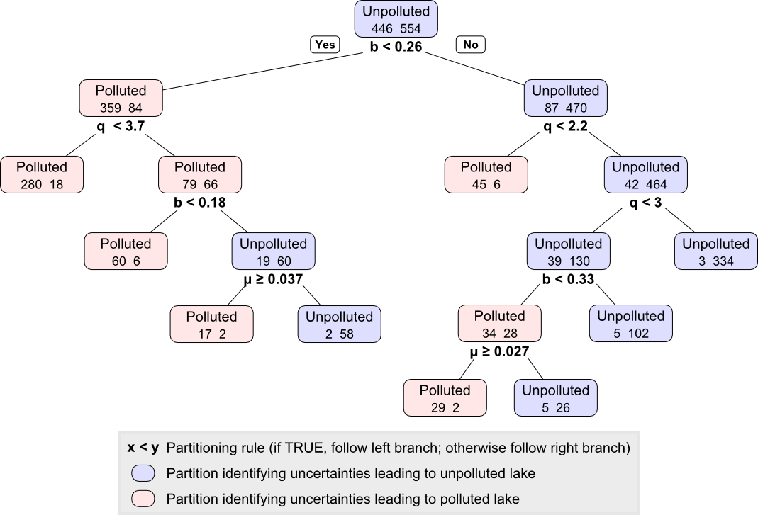
Following the rules shown in this tree, such as b < 0.26, we can develop rules that lead to Polluted or Unpolluted nodes. As with PRIM, these rules can then be used to inform the design or used as monitoring signposts.

Conclusion

In this blog post, we introduced OpenMORDM and walked through a case study using the Lake Problem.  In the end, we were able to identify key vulnerabilities that would cause the system to fail.  OpenMORDM is a library for facilitating this analysis.  Furthermore, OpenMORDM is an open source project and we encourage users to contribute bug fixes and/or enhancements.